

Introduction
Materials and Methods
Results and Discussion
토양수분 함량 (WTR) 변화양상
토양수분 함량 (WTR) 추정모형 설정
토양수분 함량 (WTR) 추정모형의 검증
월평균 강수량 및 누적강수량 추정모형 설정
월평균 강수량 및 누적강수량 추정모형의 검증
Conclusions
Introduction
토양수분 조건은 농업에서 가장 중요한 요소 중의 하나일 것이다 (David et al., 2007; Gribovszki et al., 2010). 토양수분은 강우, 관개 및 모세관 상승에 의한 유입요인과 유거, 증발산 및 지하 배수에 의한 배출요인의 결과로 산정되는 물 수지 (Blaney and Criddle, 1962; Rattan and Manoj, 2004)와 토양의 토양수분 특성 (soil water characteristic curve)에 영향받는 토양수분 이동 특성에 따라 변화한다 (Brooks and Corey, 1964; Ahuja et al., 1985; Kosugi and Hopmans, 1998; Fredlund and Xing, 1994; Eom et al., 1995; Kosugi, 1996, 1999; Rattan and Manoj, 2004; Pedroso et al., 2009; Eom, 2015; Terleev et al., 2016). 토양수분에 대하여 포장에서 측정한 raw data에 의해서만 변화 진폭이나 변화 주기성 및 급하게 변화되는 시점 (변곡점) 등을 판단하기는 매우 어렵다. 따라서 토양수분과 관련한 연구에서 토양수분 함량을 추정할 수 있는 다양한 모형개발이 매우 중요하며 개발된 모형을 통하여 변화 특성을 구명할 수 있게 된다. 모형을 개발할 경우 우선 적절한 모형의 함수 형태를 선정하고 최소제곱법 등에 의해 계수를 구한 다음 그 계수를 적용할 경우 오차의 범위가 어느 정도인가를 분석하여 그 모형이 「적절하다」라고 할 수 있는지 판단하여야 한다. 이러한 과정을 모델 검증이라고 하며 모든 모형은 반드시 모형 검증과정을 통해야만 그 모형의 적절성 여부를 판단할 수 있게 된다. 토양수분 함량 추정모형은 물 수지 모형개발, 물 관리 기술 개발 및 수량예측 모형개발 등에 필수적으로 필요한 모형이다 (Li et al., 2019). 경시적으로 토양수분 함량을 측정하기 위해서는 토양 비 파괴적인 간접적 측정방법이 사용되며 그 측정치에는 오차가 포함될 수밖에 없다. 이러한 토양수분 측정방법에 따른 토양수분 함량의 오차 분석에 관한 연구는 있으며 (Sinclair and Williams, 1979; Vauclin et al., 1984; Eom et al., 1988), 이외에도 오차 분석 방법에 관한 연구도 많이 이루어져 오고 있으나 (Goodman, 1960; Kendall and Stuart, 1963; Mandel, 1964; Shein et al., 2013; Irsyard et al., 2019; Eom et al., 2020), 일 년 이상 장기적으로 토양 깊이 별 토양수분 함량을 주기적으로 조사한 data는 찾아보기 어려웠다. 따라서 본 연구에서는 기상청에서 제공해주는 안동기상관측소에서 장기간 주기적으로 조사한 토양수분 함량에 대하여, trigonometric function, Fourier function 및 exponential function의 세 가지 형태로 추정모형을 설정하였고, 토양수분 함량에 결정적인 영향을 주는 강수량에 대하여 월평균 강수량에 대해서는 Gaussian function, 년 누적강수량에 대해서는 sigmoid function 형태의 추정모형을 설정하였으며, 설정된 총 다섯 가지 추정모형에 대하여 오차 분석 이론 (Moriasi et al., 2007; Shein et al., 2013; Irsyard et al., 2019)에 근거하여 모형을 검증하고 타 연구결과에서 개발된 모형들과의 상대적인 정밀도를 비교 검토하여, 모형 설정을 통한 토양수분 함량의 변화양상을 구명코자 실시하였다.
Materials and Methods
본 연구에 이용된 안동지역 토양 깊이 별 토양수분 함량은 2009년부터 2012년까지 4년 동안 안동기상관측소에서 표층토의 토성이 사양토이며 심층토의 토성은 사양질 계인 토양에서, 토양수분 함량 측정 센서 (규격: EASY-AG)를 이용하여 측정한 토심 10 cm, 20 cm, 30 cm 및 50 cm의 토양수분 함량 (WTR: cm3cm-3, %)을 기상자료로 공개한 data에 근거하였으며, 토심 40 cm의 WTR은 30 cm와 50 cm WTR의 평균값으로 산정하였다. 본 연구에서 WTR은 Eq. 1의 trigonometric function 형태의 모형 (TFM)과 Eq. 2의 Fourier function 형태의 모형 (FFM)을 이용하여 추정하였다.
X : 년 중 해당 순의 순서 (1-36)
yo, a, b, c : 계수
여기서, 계수 yo는 모형 전체의 값에 영향을 미치는 절편으로써 보정 계수이며 계수 a는 변화 진폭을 의미하고 계수 b는 변화 주기를 의미하며 계수 c는 변곡점의 시기를 의미하게 된다.
X : 경과 순 (elapsed 10 days)
yo, a, b, c, d, e, f, g, h, m, n : 계수
여기서, 계수 yo는 모형 전체의 값에 영향을 미치는 절편으로써 보정 계수이며 계수 a, b, e, f는 변화 진폭과 관련된 계수이고 계수 c, g, m, n은 변화 주기와 관련된 계수이며 계수 d, h는 변곡점의 시기와 관련된 계수이다.
급격한 WTR 감소에 대해서는 Eq. 3의 exponential function 형태의 모형 (EFM)을 이용하여 추정하였다.
X : 경과 순 (elapsed 10 days)
a, b : 계수
여기서, 계수 a는 변화 진폭과 관련된 계수이고 계수 b는 변화 기울기와 관련된 계수이다.
월평균 강수량은 Eq. 4의 Gaussian function 형태의 모형 (GFM)을 이용하여 추정하였다.
X : 경과 순 (elapsed 10 days)
a, b : 계수
여기서, 계수 yo는 모형 전체의 값에 영향을 미치는 절편으로써 보정 계수이며 계수 a는 최댓값을 나타내는 시기와 관련된 계수이고 계수 b는 변화 폭과 관련된 계수이다.
누적강수량은 Eq. 5의 sigmoid function 형태의 모형 (SFM)을 이용하여 추정하였다.
X : 경과 순 (elapsed 10 days)
a, b : 계수
여기서, 계수 yo는 모형 전체의 값에 영향을 미치는 절편으로써 보정 계수이며 계수 a는 변화 진폭과 관련된 계수이고 계수 b는 급증하는 시기와 관련된 계수이며 계수 c는 변화 기울기와 관련된 계수이다.
변량에 대한 범위 (range)는 Eq. 6과 같이 산정하였다.
Mmax : 최댓값
Mmin : 최솟값
NSE (nash-sutcliffe efficiency coefficient: Nash and Sutcliff, 1970)는 Eq. 7과 같이 산정하였다 (Moriasi et al., 2007, 2015; Nruthya and Srinivas, 2015; Fuamba et al., 2019).
Pi : 모형에 의한 추정치 (estimated value)
Oi : 실측치 (observed value)
Om : 실측치의 평균
Root mean square error (RMSE)는 Eq. 8과 같이 산정하였다 (Frot et al., 2008; Wang and Li, 2010; Nruthya and Srinivas, 2015; Chen et al., 2019).
Pi : 모형에 의한 추정치 (estimated value)
Oi : 실측치 (observed value)
Results and Discussion
토양수분 함량 (WTR) 변화양상
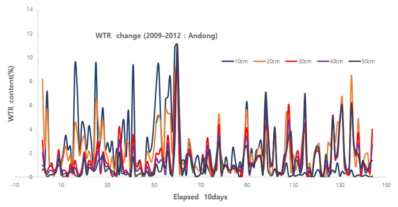
안동지역의 2009년부터 2012년까지의 토양 깊이 별 토양수분 함량 (WTR)을 나타낸 것이 Fig. 1이며, 토양 깊이 10 cm부터 50 cm까지의 평균 WTR은 10.71 (2012년) - 21.59% (2009년) 범위이었으며, 4년간의 평균 Range는 9.69%이었다 (Table 1). 토양 깊이 별 4년 평균 WTR은 8.99 (10 cm) - 18.97% (50 cm) 범위이었고 토심 간의 평균 Range는 23.4%이었으며 토양 깊이가 깊을수록 높았다 (Table 2).
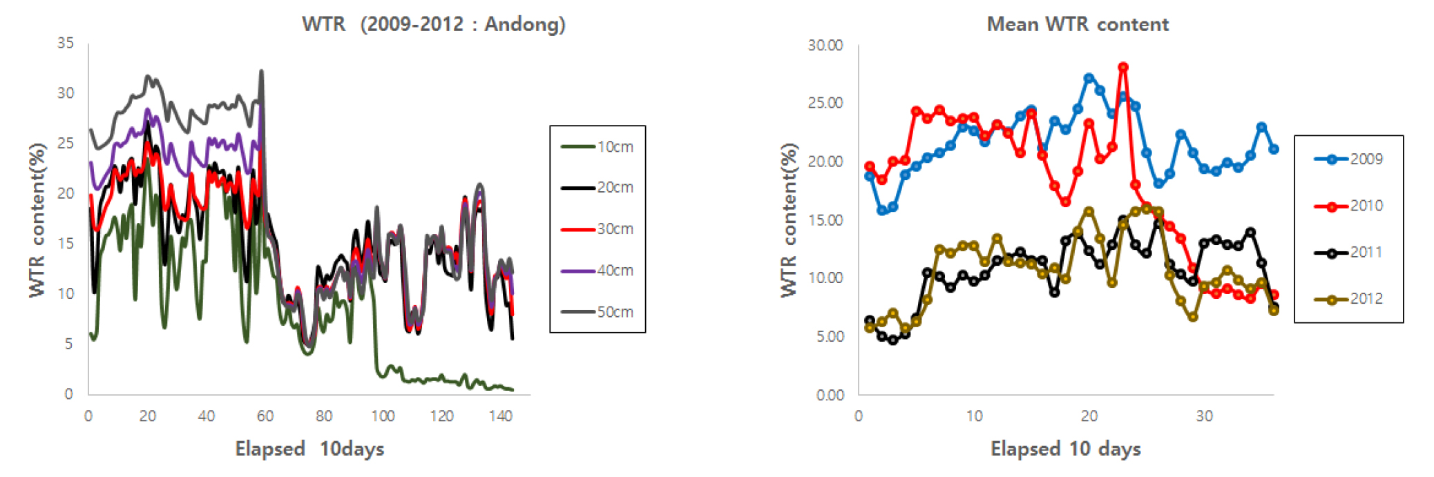
Table 1.
Statistics of average soil water (WTR) content from 10 cm to 50 cm in Andong.
Table 2.
Statistics of yearly WTR content at five kinds of soil depth in Andong.
토양수분 함량 (WTR) 추정모형 설정
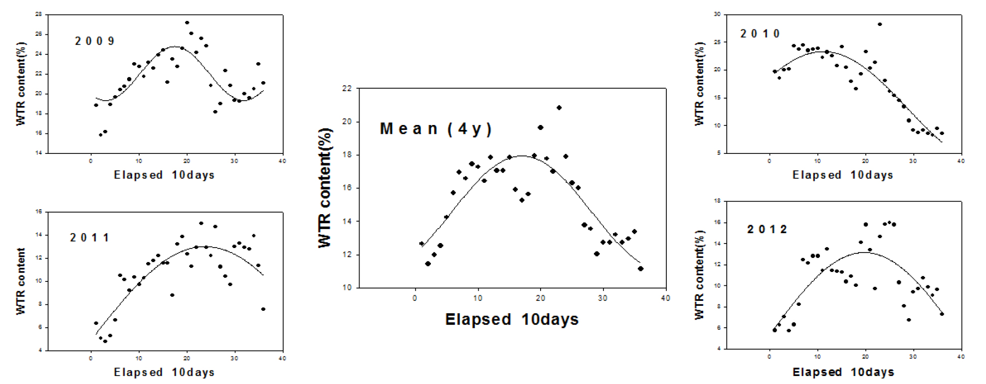
연도별 토양 깊이 10 cm부터 50 cm까지 평균 WTR에 대한 연도별 추정모형 (Fig. 2)은 각각 Eq. 9, 10, 11, 12, 13과 같이 trigonometric function (TFM) 형태로 설정되었다. 년 WTR의 변화 진폭은 5.4 (2009년) - 20.2% (2010년) 범위이었고 연도에 따른 변화 주기는 288 (2009년) - 948일 (2011년)으로서 range는 660일이었으며, 변화 변곡점 시기는 2010년이 가장 느렸고 2012년이 가장 빨랐다.
X : 경과 순 (elapsed 10 days)
토양 깊이 별 4년 평균 WTR에 대한 추정모형 (Fig. 3)은 각각 Eq. 11, 12, 13, 14, 15, 16, 17, 18, 19와 같이 trigonometric function (TFM) 형태로 설정되었다. 토양 깊이에 따른 WTR의 변화 진폭은 9.3 (20 cm) - 19.4% (50 cm) 범위이었고 변화 주기는 1,626일 (50 cm) - 2,053일 (20 cm)로서 range는 427일이었으며, 토양 깊이가 깊을수록 변화 주기는 짧았다. 변화 변곡점 시기는 토양 깊이 10 cm에서 가장 느렸고 토양 깊이 20 cm에서 가장 빨랐다.
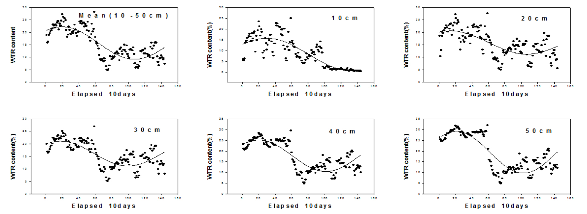
X : 경과 순 (elapsed 10 days)
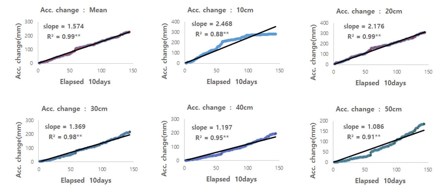
토양 깊이별 일 순 동안 변화한 WTR 양을 나타낸 것이 Fig. 4이며 4년간 누적변화량을 나타낸 것이 Fig. 5이다. Fig. 5의 slope는 일 순 동안 변화된 WTR의 변화율을 뜻하며 1.086 (50 cm) - 2.468%/10 days (10 cm) 범위이었고 10 cm부터 50 cm까지의 평균 변화율은 1.574%/10 days이었으며 토양 깊이가 깊을수록 낮았다.
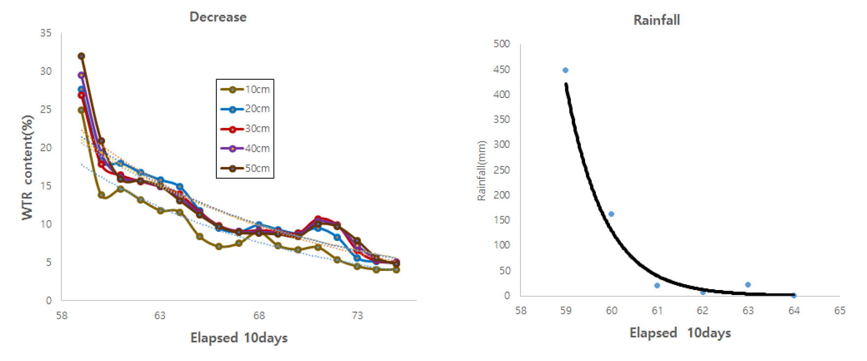
총 4년 기간 중 59 순 (2010년 8월 중순)부터 75 순 (2011년 1월 하순)까지 WTR이 급격히 감소하였는데 초기에는 토심 간 WTR의 Range는 7.10%이었으나, 약 1개월이 경과 한 후에는 2.70 - 3.60%이었으며 그 이후부터는 약 2% 정도로 낮아졌다. 이와 같은 결과는 토양 깊이별 WTR의 변이가 집중 강우 직후 경우처럼 토양수분 장력이 낮은 상태의 투수 (infiltration)가 일어나는 경우는 약 2 - 3% 및 6 - 12%로 컸으나 중력에 의해서만 투수가 일어나는 경우는 2% 및 5%로 작았다는 연구결과 (Shein et al., 2013)와 유사한 결과를 보였다. 토양 깊이별 및 10 cm부터 50 cm까지의 평균 WTR의 감소 (Fig. 6)에 대한 추정모형은 Eq. 20, 21, 22, 23, 24, 25와 같이 exponential function (EFM) 형태로 나타났으며 토양 깊이별 변화율의 지표인 지수의 값이 -0.081~-0.094 범위로서 별 차이가 없었다.
X : 경과 순 (elapsed 10 days)
토양수분 함량 (WTR) 추정모형의 검증
어떤 모형에 대한 검증을 위해서는 실측치와 모형에 의한 추정치에 대한 정밀도를 분석하여야 하며, 이 경우 결정계수 (R2: Coefficient of determination)에만 근거하여 판단하면 위험하고, 이때 추정모형의 검증에 사용되는 Data는 각각의 실측치와 모형 식에 의해 산정된 추정치와의 차이 제곱을 산정하여, 각각 Eq. 7과 Eq. 8에 의한 NSE와 RMSE를 산출해야 한다. 예를 들면 Freebairn et al. (2018)과 Maihemuti et al. (2021)은 물 수지 (water balance) 이론 (Blaney and Criddle, 1962; Williams and LaSeur, 1976)을 이용하여 토양수분 함량을 추정한 결과 측정치와 추정치 관계의 결정계수 (R2)가 높은 것으로 볼 때 통계적으로 고도의 유의성이 인정되어 추정 결과 및 Freebarirn의 연구에 사용된 model도 「적절하다」라고 판단하였다. 그러나 비록 R2값이 높다 하더라도 RMSE 및 NSE 등의 지표와 함께 판단하여야 하며, 이때 RMSE는 낮은 편이면서 NSE가 0.5 이상이어야 토양수분 등 물과 관련된 모형에 의한 추정치 또는 그 모형이 「적절하다」라고 판단하는 것이 더 합리적인 방법이라 하였다 (Moriasi et al., 2007; Shein et al., 2013; Irsyard et al., 2019). 따라서 본 연구에서도 설정된 추정모형에 대하여 「적절하다」라는 판단의 기준으로 R2과 NSE 및 RMSE에 근거하여 판단코자 한다. 이와 함께 다른 연구결과와 상대적인 정밀도의 비교 분석은 RMSE, RRA, PRE, MD, NSE 등 5개의 지표에 근거하여 다른 연구에서 제시된 지표와 비교하였다. 각 년도 별 토양 깊이 10 cm부터 50 cm까지 평균 WTR 및 4년 평균 WTR에 대한 trigonometric function 형태의 추정모형 (TFM: Fig. 2)에 의한 추정치와 실측치의 상관관계 (Fig. 7)에서 R2값이 모두 고도의 유의성이 있었고, RMSE는 1.497 - 2.440% 범위이었고 평균치에 대한 값은 1.352%로서 상당히 낮은 편이었으며, NSE는 0.510 - 0.817 범위로 평균치에 대한 값은 0.696으로서 모두 0.5 이상을 나타내었다 (Table 3). 이와 같은 결과와 「적절하다」라는 판단 기준 (Moriasi et al., 2007; Shein et al., 2013; Irsyard et al., 2019)에 근거하여 볼 때 본 TFM은 「매우 적절하다」라고 판단되었다.
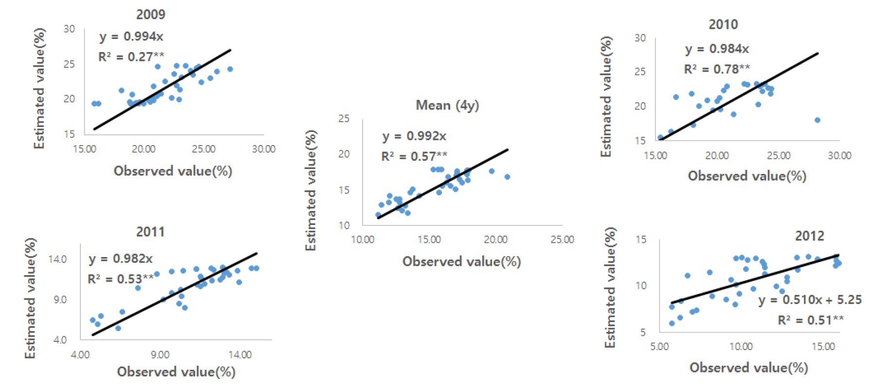
Table 3.
Performance evaluation criteria of average WTR content from 10 cm to 50 cm for trigonometric function model (TFM) calibration and validation results.
또한, 토양 깊이 10 cm부터 50 cm까지 평균 WTR의 4년 평균 WTR에 대한 또 다른 모형을 Eq. 26과 같이 Fourier function 형태로 추정모형 (FFM: Fig. 8 left)을 설정하여 검정한 결과 모형에 의한 추정치와 실측치의 상관관계 (Fig. 8 right)에서 R2값이 고도의 유의성이 있었고, RMSE는 1.944 - 3.134% 범위이었고 평균치에 대한 값은 1.356%로서 낮은 편이었으며, NSE는 0.328 - 0.698 범위로 평균치에 대한 값은 0.696으로써 0.5 이상을 나타내었다 (Table 4). 이와 같은 결과와 「적절하다」라는 판단 기준 (Moriasi et al., 2007; Shein et al., 2013; Irsyard et al., 2019)에 근거하여 볼 때 본 FFM은 「적절하다」라고 판단되었다.
X : 경과 순 (elapsed 10 days)
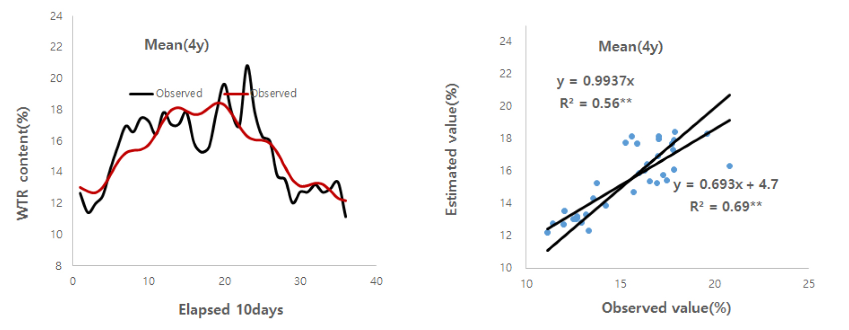
Table 4.
Performance evaluation criteria of average WTR contents from 10 cm to 50 cm for Fourier function model (FFM) calibration and validation results.
총 4년 기간 중 WTR이 급격한 감소에 대한 exponential function (EFM) 형태의 추정모형 (Fig. 6)에 의한 추정치와 실측치의 상관관계 (Fig. 9)에서 R2값이 모두 고도의 유의성이 있었고, RMSE는 1.716 - 2.995% 범위이었고 평균치에 대한 값은 2.117%로써 낮은 편이었으며, NSE는 0.778 - 0.911 범위로 평균치에 대한 값은 0.857로써 모두 0.5를 크게 상회 하는 것으로 나타났다 (Table 5). 이와 같은 결과와 「적절하다」라는 판단 기준 (Moriasi et al., 2007; Shein et al., 2013; Irsyard et al., 2019)에 근거하여 볼 때 본 EFM은 「매우 적절하다」라고 판단되었다.
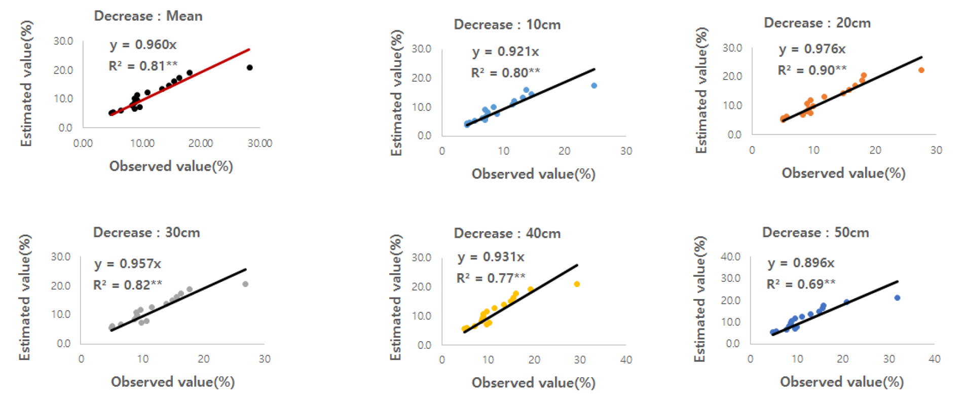
Table 5.
Performance evaluation criteria of decrease for exponential function model (EFM) calibration and validation results.
이와 같은 결과 (Figs. 2, 3, 6, 7, 8, 9 및 Tables 3, 4, 5)에 근거하여, 본 연구에서 설정한 WTR 추정모형 즉 TFM과 FFM 및 EFM을 다른 연구에서 설정한 모형들과 상대적인 정밀도를 비교해 보면, 중국 북부지역의 봄 재배 밀 포장에서 조사된 WTR에 대하여 세 가지 모델 (SWAP, HYDRUS-ID, LAWSTAC)을 이용하여 추정한 결과 세 가지 모형 모두 2007년 및 2008년의 RMSE는 각각 2.0% 및 6.0%를 나타낸 결과 (Chen et al., 2019)와 비교하여 볼 때 TFM과 FFM은 중국의 2007년 및 2008년 결과보다 정밀도가 높았고, EFM은 중국의 2007년 결과와는 근사하였으나 중국의 2008년 결과보다 정밀도가 더 높았다. 동계 밀 포장, 봄 재배 옥수수 포장, 알팔파 및 초지의 WTR에 대하여 EPIC model을 이용하여 추정한 값에 대한 RRA가 각각 18.09 - 21.97%, 10.29 - 14.31%, 55.61% 및 10.19%를 나타낸 중국의 연구결과 (Wang and Li, 2010)와 비교하여 볼 때 TFM과 FFM 모두 정밀도가 더 높았으며, EFM은 근사하였다. WCM (Baghdadi et al., 2016; Meng et al., 2016)과 SAFY (Duchemin et al., 2008; Hadria et al., 2010; Fieuzal et al., 2011; Claverie et al., 2012)을 연계하여 6회에 걸쳐 나지 WTR 측정치와 추정치 관계의 R2값은 0.15 - 0.66을 나타내었고, RMSE는 2.24 - 3.16%를 나타낸 연구결과 (Han et al., 2020)와 비교하여 볼 때 TFM, FFM 및 EFM 모두 정밀도가 더 높았다. 토양 깊이 5 cm의 WTR을 5년간 조사한 결과에 대하여 추정한 모형의 RMSE는 5.3 - 5.6%를 나타낸 연구결과 (Frot et al., 2008)와 비교하여 볼 때 TFM, FFM 및 EFM 모두 정밀도가 더 높았다. 토양 깊이 200 cm까지 약 30 cm 간격으로 3년 동안 측정한 tensiometer 측정치에 근거하여 scale factor와 hydraulic function을 이용하여 WTR을 추정한 결과 평균 PRE는 2.91 - 4.18%를 나타낸 연구결과 (Jing and Chen, 2011)와 비교하여 볼 때 TFM, FFM 및 EFM 모두 정밀도가 약간 낮았다.
월평균 강수량 및 누적강수량 추정모형 설정
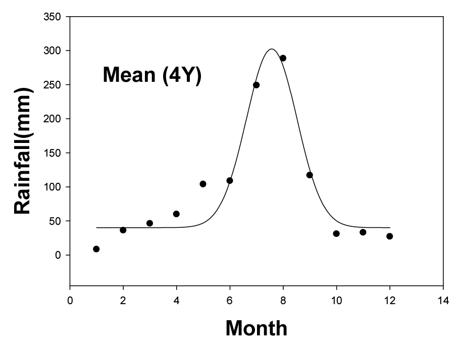
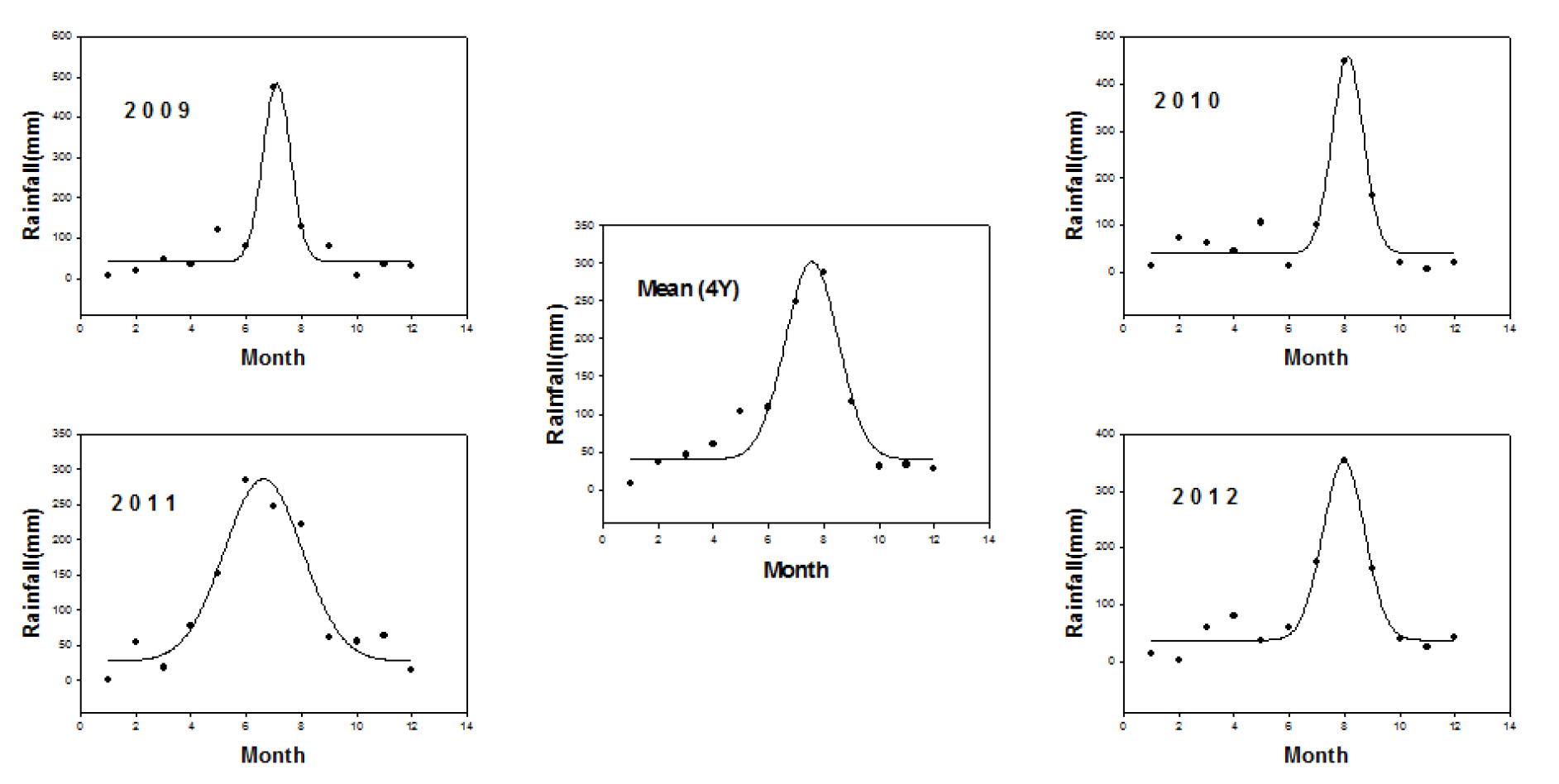
일반적으로 WTR에 가장 큰 영향을 미치는 강우 특성은 나라마다 큰 차이를 보이며, 예를 들어 스페인의 남동쪽 지역인 Almeria 주의 경우처럼 1회 강수량이 23개월 동안의 강수량에 해당하는 강수특성을 보이는 지역도 있다 (Frot et al., 2008). 본 연구 대상 지역인 안동의 경우 7 - 8월의 강수량은 연도에 따라 년 강수량의 37.5 - 57.1%를 차지하였고 4년 평균 48.5%를 차지하였다 (Fig. 10). 년도 별 월평균 강우량의 Range는 284.1 - 469.4 mm이었다 (Table 6). 월평균 강수량에 대한 추정모형을 Eq. 27, 28, 29, 30, 31과 같이 Gaussian function 형태의 추정모형 (GFM: Fig. 11)을 설정하였다.
X : 경과 순 (Elapsed 10 days)
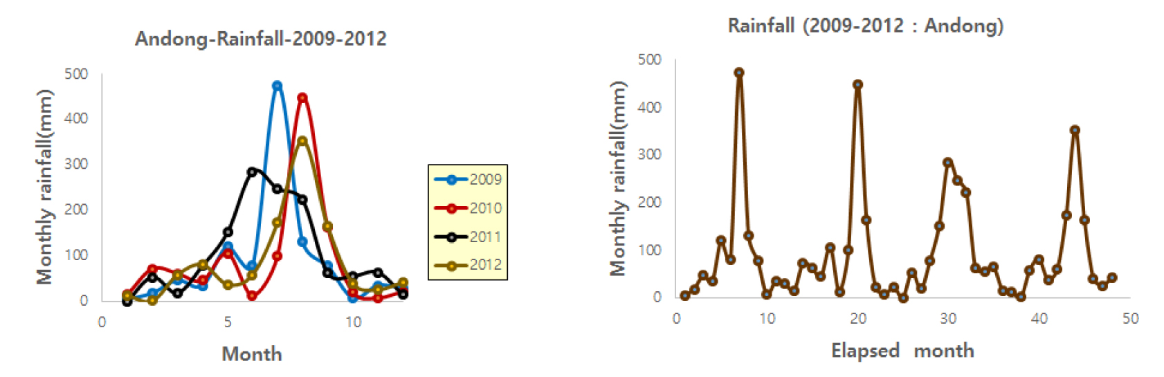
Table 6.
Statistics of monthly rainfall in Andong.
년 누적강수량에 대한 추정모형을 Eq. 32, 33, 34, 35, 36과 같이 sigmoid function 형태의 추정모형 (SFM: Fig. 12)을 설정하였다. 년 누적강수량은 2009년이 변화 기울기가 가장 높았으며, 2011년이 급증하는 시기가 가장 빨랐다.
X : 경과 순 (elapsed 10 days)
월평균 강수량 및 누적강수량 추정모형의 검증
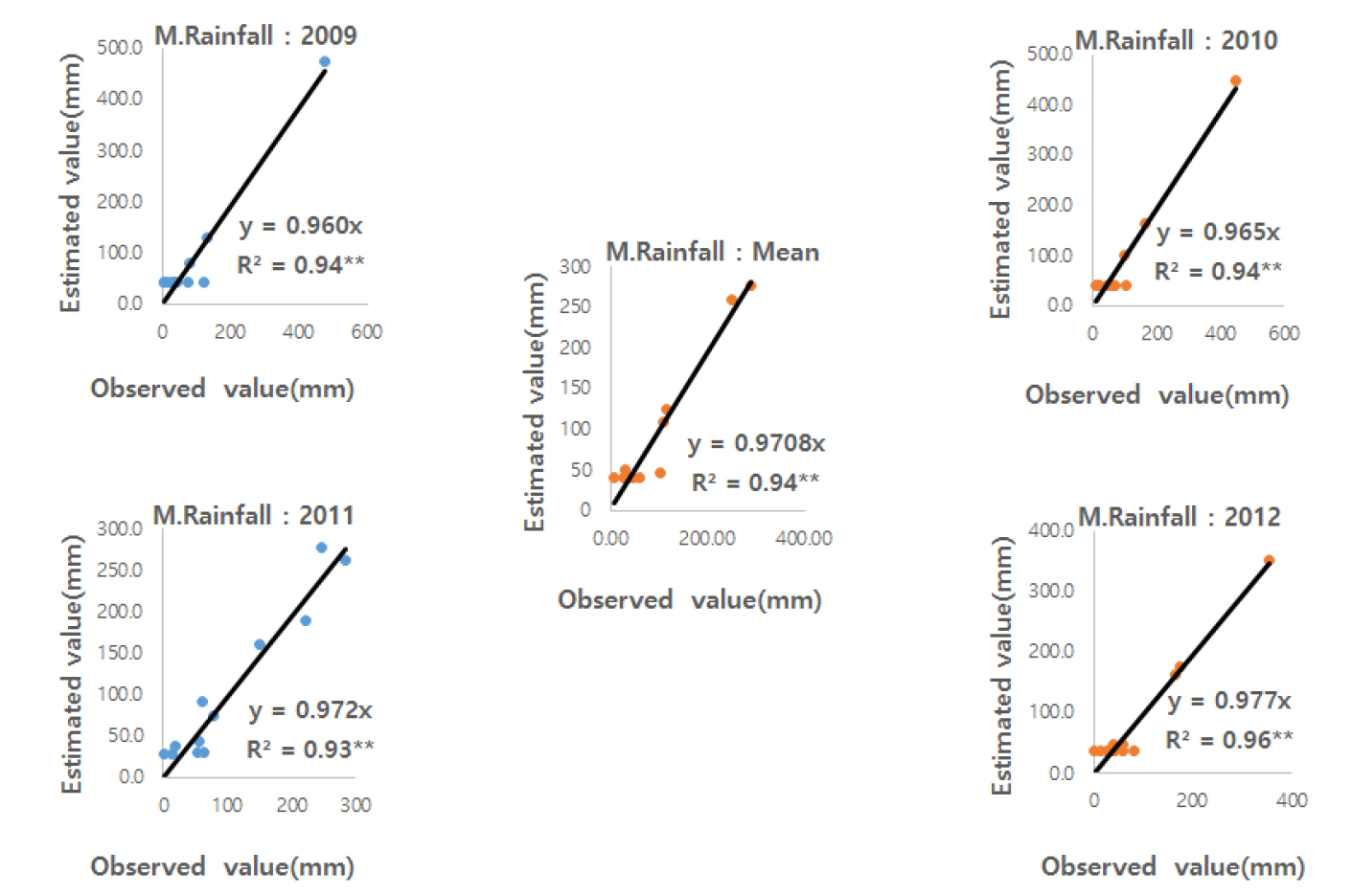
월평균 강수량에 대한 GFM에 의한 추정치와 실측치의 상관관계 (Fig. 13)에서 R2값이 모두 0.9 이상으로 매우 높았고, NSE는 0.936 - 0.958 범위로 평균치에 대한 값은 0.937로서 모두 1.0에 가까운 값을 나타내었다 (Table 7). 이와 같은 결과를 전기한 다른 연구결과 (Frot et al., 2008; Wang and Li, 2010; Jing and Chen, 2011; Chen et al., 2019; Han et al., 2020)과 비교하여 보면 GFM의 정밀도가 더 높았다. 이와 같은 결과와 「적절하다」라는 판단 기준 (Moriasi et al., 2007; Shein et al., 2013; Irsyard et al., 2019)에 근거하여 볼 때 본 GFM은 「매우 적절하다」라고 판단되었다. 년 누적강수량에 대한 SFM에 의한 추정치와 실측치의 상관관계 (Fig. 14)에서 R2값이 모두 0.98 이상으로 매우 높았으며, NSE는 0.976 - 0.999 범위로 평균치에 대한 값은 0.996으로서 모두 1.0에 가까운 값을 나타내었다 (Table 8). 이와 같은 결과를 전기한 다른 연구결과 (Frot et al., 2008; Wang and Li, 2010; Jing and Chen, 2011; Chen et al., 2019; Han et al., 2020)와 비교하여 보면 SFM의 정밀도는 매우 높았다. 이와 같은 결과와 「적절하다」라는 판단 기준 (Moriasi et al., 2007; Shein et al., 2013; Irsyard et al., 2019)에 근거하여 볼 때 본 SFM은 「매우 적절하다」라고 판단되었다.
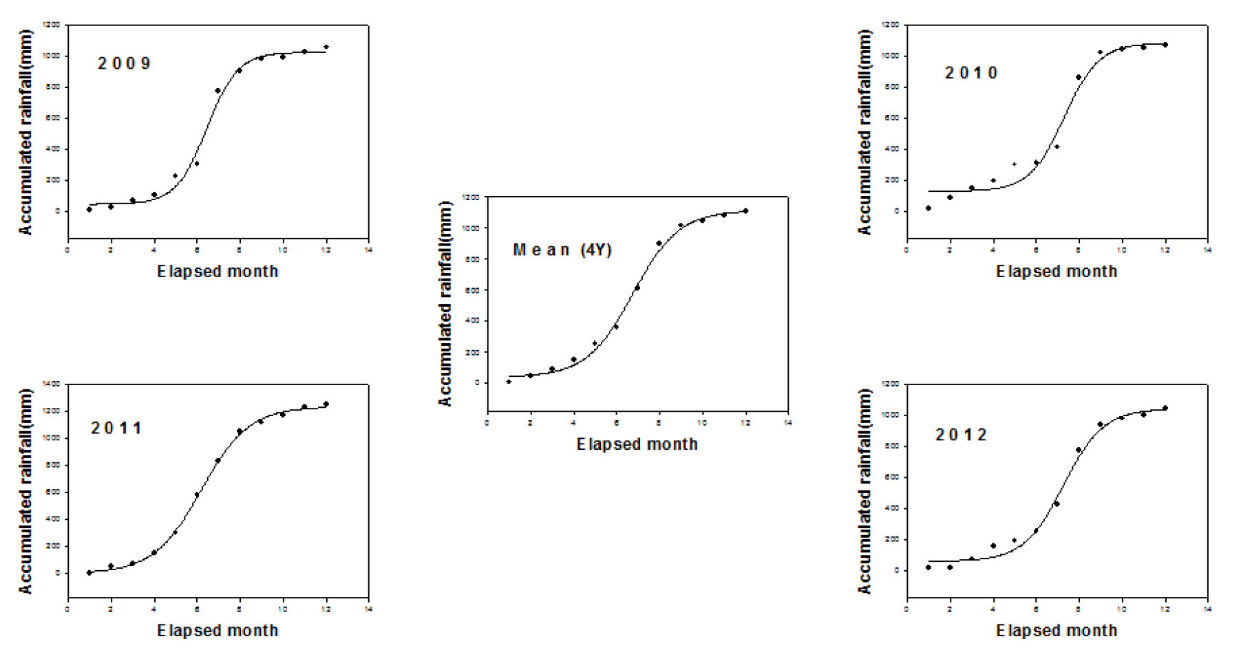
Table 7.
Performance evaluation criteria of monthly rainfall for Gaussian function model (GFM) calibration and validation results.
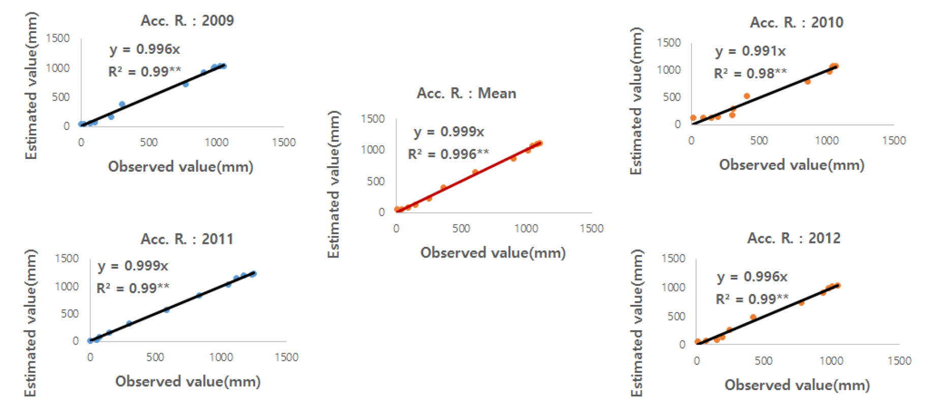
Table 8.
Performance evaluation criteria of accumulated rainfall for sigmoid function model (SFM) calibration and validation results.
이상의 결과로 볼 때, 본 연구에서 설정한 5가지 모형의 상대적인 정밀도는 추정치와 실측치 상관관계의 R2값을 기준으로 삼을 때는 SFM > GFM > EFM > TFM > FFM 순으로, RMSE를 기준으로 삼을 때는 TFM > FFM > EFM > GFM > SFM 순으로, NSE를 기준으로 삼을 때는 SFM > GFM > EFM > TFM > FFM 순으로 정밀도가 높았다. 즉 RMSE를 기준으로 삼을 때는 강수량 추정모형보다 WTR 추정모형이, NSE를 기준으로 삼을 때는 WTR 추정모형보다 강수량 추정모형이 상대적으로 정밀도가 더 높았다. 결론적으로 보면, 본 연구에서 설정한 5가지 모형의 결과와 「적절하다」라는 판단 기준 (Moriasi et al., 2007; Shein et al., 2013; Irsyard et al., 2019)에 근거하여 볼 때 본 연구에서 설정된 4가지 모형 (TFM, EFM, GFM, SFM)은 「매우 적절하다」라고 판단되었으며, FFM은 「적절하다」라고 판단되었다.
Conclusions
안동지역을 case study 하여, 2009년부터 2011년까지 토양 깊이 10 cm부터 50 cm까지 10 cm 간격으로 조사된 순 (10일) 평균 토양수분 함량 (WTR)과 월평균 강수량 및 년 누적강우량을 대상으로 하여, 각 년도 별 토양 깊이 10 cm부터 50 cm까지 평균 WTR 및 토양 깊이 별 4년 평균 WTR에 대해서는 trigonometric function 형태의 모형 (TFM)과 Fourier function 형태의 모형 (FFM), WTR의 급격한 감소에 대해서는 exponential function 형태의 모형 (EFM), 월평균 강수량에 대해서는 Gaussian function 형태의 모형 (GFM), 년 누적강수량에 대해서는 sigmoid function 형태의 모형 (SFM) 등 총 다섯 가지의 추정모형을 설정하였다. 토양 깊이 50 cm까지의 평균 WTR의 변화 진폭은 12.64%이었다. 연도에 따른 변화 주기의 range는 660일이었고, 토양 깊이에 따른 변화 주기의 range는 427일이었으며, 토양 깊이가 깊을수록 변화 주기는 짧았다. 년 누적강수량은 2009년이 변화 기울기가 가장 높았으며, 2011년이 급증하기 시작하는 시기가 가장 빨랐다. 모형의 RMSE는 TEM, FFM, EFM, GFM 및 SFM 각각 1.352%, 1.356%, 2.117%, 21.37 mm, 및 27.09 mm이었으며, NSE는 각각 0.696, 0.694, 0.857, 0.937 및 0.996이었다. 본 연구에서 설정한 5가지 모형의 검증 결과와 「적절하다」라는 판단 기준 (Moriasi et al., 2007; Shein et al., 2013; Irsyard et al., 2019)에 근거하여 볼 때 본 연구에서 설정된 4가지 모형 (TFM, EFM, GFM, SFM)은 「매우 적절하다」라고 판단되었으며, FFM은 「적절하다」라고 판단되었다.
