

Introduction
Materials and Methods
Study area
Soil data and laboratory analysis
Estimation of bulk density
Calculation of soil organic carbon density and carbon stocks
Environmental covariates
Equal-area spline profile function
Spatial predict model and validation
Results
descriptive statistics and estimated bulk density
Importance of covariate in predicting SOC stock
Validation of Cubist model prediction
SOC stock
Conclusions
Introduction
Soil organic carbon (SOC) is the essential nutrients for plant growth and major components of the global carbon cycle (Batjes, 1996). SOC affect the concentration of greenhouse gases in the atmosphere and global climate changes (Powers and Schlesinger, 2002). SOC has the ability to improve the soil physical, chemical, and biological properties, which can enhance soil security. Soil has 1,500 Gt C in the top one meter, globally (Jobbágy and Jackson, 2001) which is approximately three times as much C found in the biosphere and twice as much C found in the atmosphere. Accurate quantification of SOC is important for assessing the C sink capacity of soils and the changes rate of SOC (Yang et al., 2009).
Digital soil mapping is the creation and population of spatial soil information systems by the use of field and laboratory observational methods coupled with spatial and non-spatial soil inference systems (Lagacherie and McBratney, 2006). Digital soil mapping does not just produce a paper map; it is a dynamic process in essentially a spatial database of soil properties, based on a sample of landscape at known locations (Mcbratney et al., 2003). Field sampling is used to determine spatial distribution of soil properties, which are mostly measured in the laboratory. These data are then used to predict soil properties in areas not sampled. Spatial variability data are important for estimating the stock of soil carbon and also for understanding the biophysical processes that can influence the flow of organic carbon in soils. Digital soil maps describe the uncertainties associated with such predictions and, when based on longitudinal data can, provide information on dynamic soil properties.
Predictions of soil organic carbon stock in digital mapping are based on relationship among soil properties and environmental factor. McBratney et al. (2003) generalized and formulated a equation, with the objective of modeling the variables responsible for the processes of soil formation through an empiric quantitative description of the relationships among other environmental covariates, used as spatial prediction functions.
This is the called the scorpan model and this function with following seven factors: = soil and other properties of the soil in a given location; = climate, climatic properties; = organisms, vegetation, = topography, attributes of the landscape; = parent material, lithology; = age, time factor; = space, spatial location; = autocorrelated random spatial variation. Each factor is represented by a group of one or more continuous of categorical variables; for example, r for elevation, slope or other derived attribute of a DEM.
The objectives of this study were to estimate soil carbon stock at two soil depth (0 - 30 cm, 0 - 100 cm) at national scale using the digital soil mapping skill.
Materials and Methods
Study area
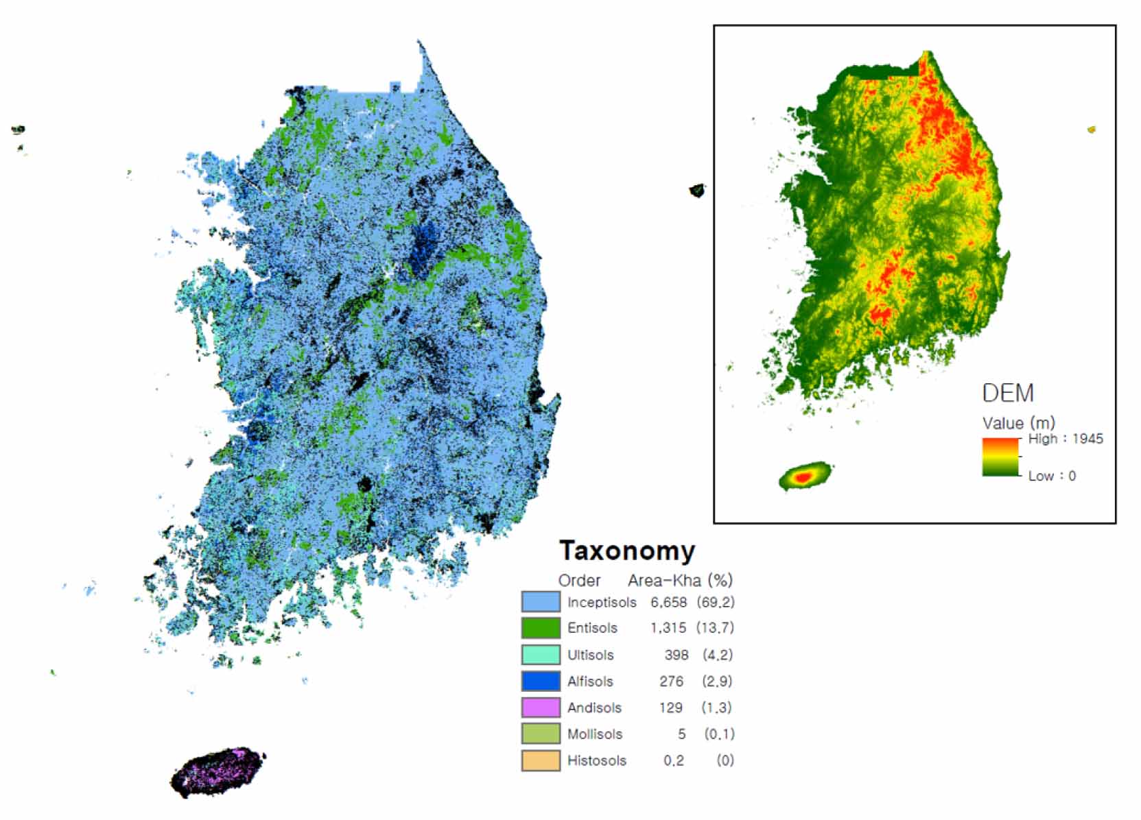
South Korea is a country in East-Asia, constituting the southern part of the Korean Peninsula. Its total area is approximately 100,000 km2 and 66% forest land and 19% agricultural land. In the humid temperate climatic condition, national mean annual precipitation (MAP, mm) and temperature is 1,300 mm, 23°C. The basis of parent rock is the granite gneiss (32.4%), granite (22.3%), schist (10.3%), limestone (10.1%). Inceptisols is constituted 69.2 percent of the Soil taxonomic system and there are 7 classes of Soil Order (RDA, 2011). Jeju island, however, is constituted basalt of Andisols class (Fig. 1).
Soil data and laboratory analysis
The original soil data (n = 5,023, 78,148 layer) was collected by Korean Rural Development Administration (RDA) from 1968 to 1990. The data includes chemical and physical properties such as soil texture, organic matter, and a limited number of gravel and bulk density contents. So we match the Korean soil map (RDA)’s location using the soil series. Finally, we selected approximately 78,148 soil layer data and used for Digital soil mapping. The location of soil sample based on soil profiles in “Taxonomical Classification of Korean Soils” (RDA, 2011). The organic matter analyzed by Turine method and multiply using 1.724 conversion factor to calculate soil organic carbon. Bulk density was calculated the mass of an dried sample of soil per unit bulk volume.
Estimation of bulk density
According to before study (Hong et al., 2013), we predict mineral bulk density (BDmin) using pedotransfer functions (PTFs) from sand content and depth based on the limited data in the database (Tranter et al., 2007).
The influence of organic matter on bulk density is then calculated based on Adams (1973)’ model.
where, organic matter is the mass percentage of organic matter (g 100 g-1), and BDOM = average organic matter bulk density = 0.224 g cm-3, and BDmin is the mineral bulk density g cm-1).
Because of the different mineralogical composition of andisols a separate model that predicted BD from OM content was derived from the Tempel et al. (1996).
Calculation of soil organic carbon density and carbon stocks
Although SOC density and SOC stock are often used interchangeably in literature (Minasny et al., 2006), they differ in scale and unit. SOC density is the SOC mass per unit area for a given depth which can be calculated as:
where, is the Bulk density (g cm-3) and, is Carbon concentration (g kg-1), is the thickness (cm) and is the gravel and stone content (%).
SOC stock is the actual SOC mass for a given soil depth and area. It was calculated by summing up the product of mean SOC density per grid and the number of grid.
where, is SOC density (ton C ha-1), is area of grid cell and 10-3 is conversion factor.
Environmental covariates
Environmental variables were selected to represent the key soil-forming factors of climate, parent material, relief and age based on the scorpan model (McBratney et al., 2003). Temperature affects the accumulation rate of carbon in soil, and temperature variables are widely used in prediction of SOC (Jobbágy and Jackson, 2000). Mean annual temperature (MAT) and mean annual precipitation (MAP) over thirty years (1970 - 2000) of the study area was obtained from Korea Meteorological Administration. These climate data collected from 67 sampling site in study area and reanalyzed and resampling to make 30 × 30 m grid layer.
Topography dataset came from the digital elevation model provided by the National Geographic Information Institute (http://air.ngii.go.kr/gis/gisSrchInfoView.do). Slope gradient, Analytical Hillshading, Topographic wetness index (TWI), Terrain ruggedness index (TRI), Topographic openness, and Mid slope position (MSP) multi-resolution index were derived from the DEM using the System for Automated Geoscientific Analysis (SAGA) software (http://www.saga-gis.org/en/index.html). Soil texture divide by 7 classes such as Sandy, Coarse_loamy, Coarse_silty, Fine_loamy, Fine_silty, Clay. Soil parent divided by the Acidic (igneous_rocks), Neutral (igneous_rocks), Basic (igneous_rocks), Volcanic_ash, Sedentary rocks, Tertiary, Quaternary, Metamorphic_rocks, extra. Relationships among SOC and BD with the environmental variables are presented in Table 1.
Table 1.
Description of environmental covariate.
Equal-area spline profile function
The spline function is based on the quadratic spline model of Bishop et al. (1999). This function was fitted to the profile values of the target soil organic carbon and bulk density using the es-splineTool of ithir package from R software to convert to horizon-based value to the IPCC standard depth (0 - 30 cm). The smoothing parameter lambda chosen was 0.1 (Malone et al., 2009).
Spatial predict model and validation
To predict spatial distribution of 0 - 30 cm SOC stock in South Korea, we applied Cubist predict model. The Cubist model is currently a very popular model. Its popularity is due to its ability to ‘mine’ non-linear relationships in data (Malone et al., 2017). This model is based on the M5 algorithm of Quinlan (1987), and is implemented in the R cubist package.
In order to calibrate SOC predict model, the splined data were randomly split into 75% for training the model, and 25% data for validation. For validation the model, validated with 30% of the data using 3 statistical parameters: R2, MAE, RMSE. The R2 is the coefficient of determination of linear regression (Eq. 7), between the observed values and predicted values. MAE is the mean error the absolute prediction error (MAE) and RMSE correspond to root mean square error (Eq. 8, Eq. 9).
where, and are predicted and observed SOC stock at site i: is the number of samples; is the Pearson correlation coefficient between the observed and predicted values.
For the uncertainty we used bootstrap model prediction on the validation data. We estimate the confidence interval of those prediction for each point.
Results
descriptive statistics and estimated bulk density
Equal-area splines (R package) modeled the depth-wise distribution and generated a continuous SOC and BD profile 0 - 100 cm depth. SOC content was highly variable and ranged from 5 to 226 ton C ha-1 for the 0 - 30 cm and from 11 to 917 ton C ha-1 in the 0 - 100 cm (Table 2). The mean SOC at 0 - 30 cm was 46 ton C ha-1 and that for the 0 - 100 cm was 102 ton C ha-1. The mean SOC for the 0 - 30 cm is almost half of 0 - 100 cm depth. Also BD was on average at a depth is 1.15 g cm-3 and 1.22 g cm-3 respectively.
Because of mineralogical difference, we used two equation for estimate bulk density (Eq. 2, Eq. 3).
Table 2.
Descriptive statistics of soil organic carbon stock (ton C ha-1) and bulk density (g cm-3).
| Parameter | Depth | Mean | SD | Min | Max | Range |
| SOC stock | 0 - 30 | 46 | 41 | 5 | 226 | 221 |
| BD | 1.15 | 0.19 | 0.56 | 1.45 | 0.88 | |
| SOC stock | 0 - 100 | 102 | 109 | 11 | 917 | 906 |
| BD | 1.22 | 0.18 | 0.57 | 1.51 | 0.94 |
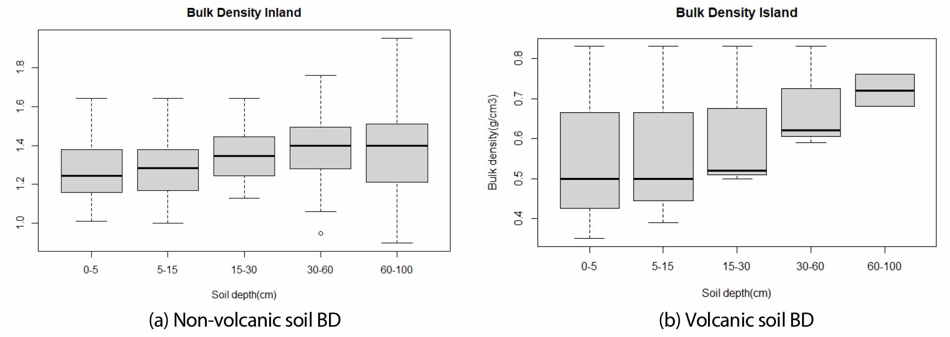
The boxplot of estimated Bulk density shown Fig. 2. In both soil type inland soil (non-volcanic) and island soil (volcanic), the estimated Bulk density value increase with the depth of the soil.
Importance of covariate in predicting SOC stock
As shown in Table 3, the Cubist, based on the whole data set (78,148 layer data), used Texture, Parent, DEM and PRCP as conditions to perform the Cubist for SOC stock for 0 - 30 cm detph. However, TRI, PRCP, DEM, TOP, TON, TWI, MSP, Tavg, TON, DAH, Hillshading and ValleyDepth were used as environmental covariates to predict the SOC stock. Among the environmental covariates, MAP, DEM, TWI, TRI, TOP, Slope and PRCP showed more influence on SOC and their spatial distributions.
Table 3.
Usage (%) of covariates in the Cubist model for predicting SOC.
Validation of Cubist model prediction
The overall cubist prediction for both depths (0 - 30 and 0 - 100 cm) is good with mean R2 of 0.78 and 0.62, respectively (Table 4). When compared between two depths the cubist did better in predicting 0 - 30 cm than 0 - 100 cm SOC stock.
Table 4.
Validation results of Cubist in predicting SOC in 0 - 30 cm and 0 - 100 cm depth.
The performance of cubist SOC stock model, R2 ranged so stability from 0.77 to 0.79 for 0 - 30 cm and 0.62 - 0.64 for 0 - 100 cm. The variation of R2 for SOC stock from cubist model, it is due to random selection effect of calibration and validation datasets.
The mean RMSE for 0 - 30 cm SOC stock and 0 - 100 cm SOC stock was 19.5 and 68.7, respectively. The 0 - 100 cm SOC stock RMSE higher than 0 - 30 cm SOC stock.
SOC stock
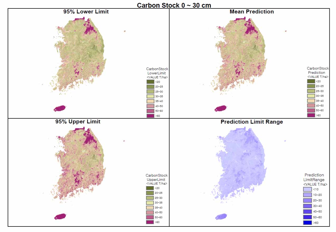
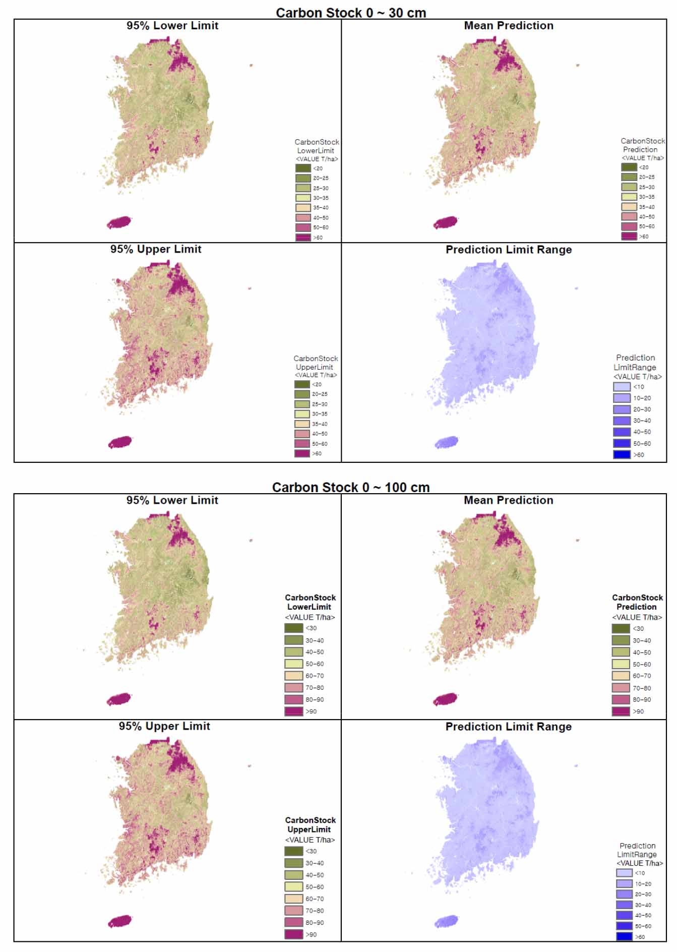
The average SOC stocks calculated for two soil depths, it was 35.2 ton C ha-1 for 0 - 30 cm and 87.1 ton C ha-1 for 0 - 100 cm depth (Table 5). In the SOC stock map, for top 30 cm soil depth, most of the country area had SOC stocks below 40 ton C ha-1 and some of mountain areas and Jeju island parts of the country have more than 50 ton C ha-1 (Fig. 3). The total SOC stock (top 1 m soil depth) map also showed similar distribution to top 30 cm SOC map, but the overall SOC stock was high.
Table 5.
Predicted mean SOC stock (ton C ha-1) and confidence interval (95%).
Conclusions
Digital Soil Mapping (DSM) can be defined as the creation and population of spatial soil information systems by numerical models inferring the spatial and temporal variations of soil types and soil properties from soil observation and knowledge and from related environmental variables (Lagacherie and McBratney, 2006). This study predicted the spatial distribution of SOC stock at two soil depth intervals (0 - 30, 0 - 100 cm) and quantified its stock (ton C ha-1) for national scale. The mean estimated SOC stock at 0 - 30 cm soil depth was 35.2 ton ha-1 and for 0 - 100 was 87.1 ton ha-1. The SOC stock map could be used for future soil organic carbon stock and predicting potential SOC sequestration.
