Original research article

Korean Journal of Soil Science and Fertilizer. 28 February 2022. 58-70
https://doi.org/10.7745/KJSSF.2022.55.1.058

ABSTRACT


MAIN

  • Introduction

  • Materials and Methods

  •   Random Forest 모델

  •   간척지 토양 데이터

  •   Random Forest 모델 검증

  • Results and Discussion

  •   Random Forest 모델의 정확도

  •   토양 탄소 함량 예측에 대한 주요 토양 특성 변수

  • Conclusions

Introduction

농경지 토양의 탄소는 대부분 유기물의 형태로 존재하여 토양의 양분 순환, 수분 유효도, 토양 구조 안정성 등 토양의 비옥도와 생산성 유지를 위한 중요 관리 항목이다 (Schmidt et al., 2011). 최근, 전 세계적으로 기후변화에 따른 식량안보 등의 문제가 심화하면서 우리나라를 포함한 세계 각국에서 농업분야에서의 온실가스 배출 저감을 위한 하나의 방안으로 토양 탄소 격리가 주목받고 있다 (Nguyen et al., 2022). 육상 생태계의 가장 큰 탄소 저장고인 토양은 대기 중 탄소의 약 2배에 달하는 양 (1,400 - 2,300 Pg C)의 탄소를 저장하고 있어 (Lal, 2008; Smith, 2012), 토양 탄소 함량 변화는 대기 이산화탄소 (CO2) 농도에 직접 영향을 준다 (Wang et al., 2022).

따라서, 우리나라에서도 농업환경변동조사 사업 등을 통해 논 (Hwang et al., 2019), 밭 (Ahn et al., 2020; Lee et al., 2020), 과수원 (Ahn et al., 2020; Kim et al., 2021) 등 농경지 유형별 토양 탄소 함량을 조사하고 있다. 토양 탄소 함량은 기본적으로 기후, 식생, 지형 등 토양 생성 요인에 영향을 받지만 (Wiesmeier et al., 2019), 농경지에서는 투입되는 유기물의 종류와 양 (Karhu et al., 2012), 그리고 토양 유기물의 물리화학적 안정화와 관련된 토양 특성 (토성, pH, 점토 함량 등) (Wiesmeier et al., 2019; Park et al., 2022)에 의해서도 영향을 받는다. 따라서, 우리나라 농경지 토양의 탄소 함량 분포를 이해하기 위해서는 다양한 유형의 토양에 대한 조사가 필요하다. 이러한 측면에서, 우리나라 전체 농경지의 10% 이상을 차지하고 있는 간척지 토양의 탄소 함량에 대한 연구 결과가 부족한 점은 아쉬운 측면이 있다 (Park et al., 2022).

우리나라 서남해안에 주로 분포하고 있는 간척지는 조성 연대에 따라 다소 상이하지만, 전반적으로 토양 탄소 함량이 낮은 편이다 (Lim et al., 2020). 특히, 간척지와 같은 염해 토양은 비염해 토양에 비해 ECe (saturated-paste electrical conductivity; 포화침출액 전기전도도)와 ESP (exchangeable sodium percentage; 치환성나트륨백분율) 등 염류 특성이 불량하기 때문에 특별한 관리가 없는 한 낮은 작물 생산성으로 토양에 투입되는 작물 잔사 유기물이 적어 결과적으로 일반 토양보다 탄소 함량이 낮다 (Lim et al., 2020). 하지만, 이는 간척지 토양의 탄소 격리능이 크다는 의미이기도 한다. 따라서, 간척지 토양의 토양 환경 개선을 통한 생산성 향상과 기후변화 저감을 위한 탄소 저장고로서의 기능을 평가하기 위해서 간척지 토양의 탄소 함량 변화 예측이 필요하다.

토양 탄소 함량은 다양한 요인에 의해 영향을 받기 때문에 탄소 함량 변화 요인을 정밀하게 평가하기가 쉽지 않다 (Nguyen et al., 2022). 따라서, 다양한 환경요인을 고려한 토양 탄소 함량 예측 기법 개발이 요구되고 있는데, 지금까지 많은 선행 연구에서는 토양 탄소 함량 예측 및 평가를 위해 선형회귀모형을 이용하였다 (Chaplot et al., 2001; Florinsky et al., 2002; Powers and Schlesinger, 2002; Thompson and Kolka, 2005; Thompson et al., 2006). 선형회귀분석은 적용과 해석이 쉽다는 장점이 있지만, 변수 사용에 대한 제약이 있어 다양한 변수에 의해 비선형적으로 복잡하게 영향을 받는 토양 탄소 함량을 예측하는 데 정확도가 낮은 경향이 있다 (Franklin, 2005). 이러한 제약을 해결하고 예측의 정확도를 높이기 위해 최근 기계학습 기반의 Random Forest 모델이 이용되고 있다 (Grimm et al., 2008; Kim and Grunwald, 2016; Nabiollahi et al., 2019; Zhou et al., 2020; Sothe et al., 2022; Zeraatpisheh et al., 2022). 우리나라에서는 Jeong (2018)이 Random Forest 모델을 이용하여 지형, 식생, 토성 및 토지이용에 따른 토양 탄소 저장량을 예측하고, 전자토양도를 이용하여 농업 경관에서 토양 탄소 저장량의 가치를 평가한 바 있다. 또한, Lee et al. (2015)는 토지피복변화에 따른 산림 탄소 저장량 분석을 위해 Random Forest 모델을 활용한 바 있다.

하지만, 현재까지 기후-지형-식생이 동일한 농경지를 대상으로 토양의 다양한 이화학성을 매개변수로 활용하여 Random Forest 모델 구현을 통해 토양 탄소 함량을 예측한 연구는 아직까지 없다. 또한, 일반 농경지 토양과 특성이 매우 상이한 간척지 토양을 대상으로 하여 Random Forest 모델을 활용한 토양 탄소 함량 예측 연구 역시 전무하다. 따라서, 본 연구에서는 우리나라의 주요 간척지 토양 특성 조사 결과를 활용하여 간척지 토양의 탄소 함량 예측을 위한 Random Forest 모델 적용 가능성을 평가하고자 하였다. 비록 토양 탄소 함량은 다양한 요인에 의해 영향을 받지만, 본 연구에서는 염해 토양인 간척지 토양 특성을 고려하여 Random Forest 모델을 이용한 토양 탄소 예측에 ECe와 ESP 등 염해 특성의 기여도가 높을 것으로 가설을 세웠다.

Materials and Methods

Random Forest 모델

Random Forest 모델은 다수의 의사결정 나무 (tree)를 임의적으로 학습하여 각각의 예측 결과를 종합하여 정확도를 높이는 앙상블 모델 중 하나이다 (Breiman, 2001) (Fig. 1). 특히, Random Forest 모델은 기계학습 기반의 모델 중에서도 과적합 (overfitting, 주어진 케이스만을 과도하게 학습하여 특이 케이스에 대처하지 못하는 현상) 문제를 방지하여 예측력이 높고, 다양한 독립변수를 사용하여 예측했을 때에도 정확도가 높다는 장점이 있다 (Breiman, 2001).

기계학습 기반의 Random Forest 모델은 Python에서 ‘sklearn’ 패키지로부터 분류 (random forest classifier) 또는 회귀 (random forest regressor) 모듈을 추출하여 구동할 수 있다. Random Forest 패키지 외에도 데이터 불러오기 및 모델 검증을 위한 통계 분석, 결과 시각화 등을 위하여 ‘pandas’, ‘numpy’ 등의 패키지를 이용할 수 있다. Random Forest 분류와 회귀 모듈 모두 결과를 예측하는 데 활용되지만, 다수 의사결정나무 각각의 예측 결과를 종합하는 방식에 차이가 있다 (Breiman, 2001). 분류 모듈의 경우 각각의 예측 결과를 투표 (다수결의 원칙)를 통해 종합하여 최종 결과를 결정하기 때문에, 예측하고자 하는 변수가 ‘예/아니오’와 같은 범주형일 때 적합하다. 토양 탄소 함량과 같이 변수의 값이 다양한 연속형일 경우에는 평균화를 통해 각각의 예측 결과를 종합하여 최종 결과를 도출하는 회귀 모듈이 적합하다 (Breiman, 2001). Python에서 Random Forest 회귀 모듈 추출 및 데이터 입력, 모델 구동 등의 코딩 과정은 다소 복잡한 편이므로 명령어에 대한 학습이 필요하다 (Table 1).

Random Forest 모델은 의사결정 나무들 사이의 상관 관계를 줄이고 예측의 정확도를 높이기 위해 일반적으로 사용되는 데이터의 70% 또는 80%를 무작위 추출하여 학습하고, 나머지 데이터를 이용하여 검증한다 (Breiman, 2001). 또한, 다양한 하이퍼 파라미터 (hyper parameter; 모델 구동을 위해 설정해주는 값)를 이용하여 예측의 정확도를 높일 수 있다 (Breiman, 2001) (Table 1). 모델의 예측 정확도 향상을 위한 하이퍼 파라미터의 최적값은 임의로 지정한 뒤 모델 구동 및 검증을 반복하여 찾거나 Python ‘sklearn’ 패키지의 ‘GridSearchCV’ 모듈을 이용하여 찾을 수 있다.
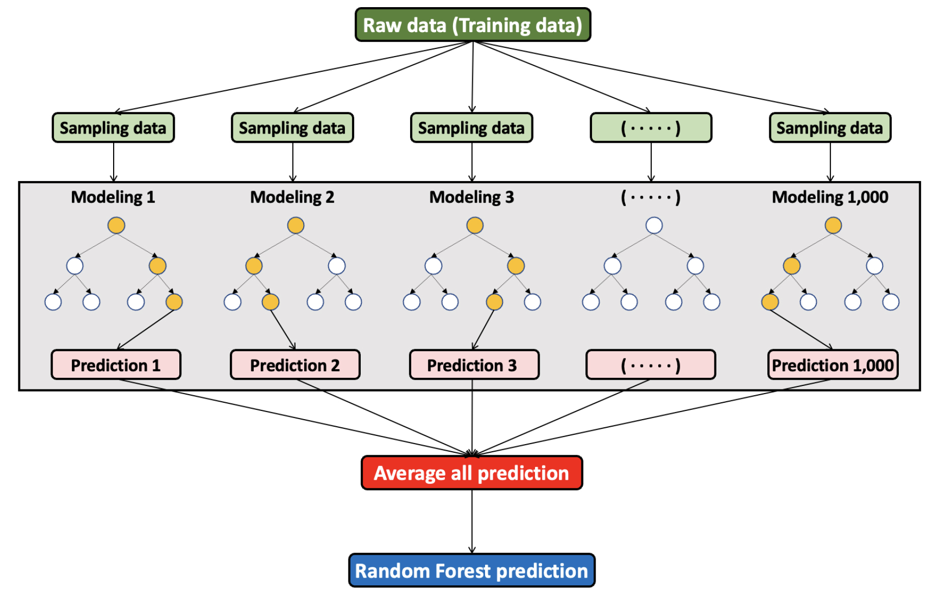
https://static.apub.kr/journalsite/sites/ksssf/2022-055-01/N0230550107/images/ksssf_55_01_07_F1.jpg
Fig. 1.

Structure and process of random forest models.

Table 1.

List of Python command for random forest regressor modeling.

Contents Command in Python Remarks
Open the package
and module
> import pandas as pd
> import numpy as np
> from sklearn.model_selection import train_test_split
> from sklearn.ensemble import RandomForestRegressor
> from sklearn.metrics import mean_squared_error
> from sklearn.metrics import r2_score
Open data > rawdata=pd.read_excel(‘folder path/file’s name.xlsx’,
usecols=‘range of columns to use’)
Specify
independent
and dependent
variables
> X=rawdata.drop([‘name of dependent variable’],
axis=1)
> X.values
> y=rawdata[‘name of dependent variable’]
> y.values
1. ‘axis’: The number of the row in which
the variable name is written in the Exel
file
2. ‘.values’: transformation data into
suitable for use in random forest model
Separation of
training and
validation data
> X_train, X_test, y_train, y_test = train_test_split(X, y,
test_size=0.2, random_state=0)
1. ‘test_size’: set the ratio to be split into
training and validation data
2. ‘random_state’: designation a number
for model reproducibility
Running random
forest regressor
model
> rf=RandomForestRegressor(random_state=0,
n_estimators=4, max_depth=3, min_samples_leaf=1,
min_samples_split=0.15)
1. ‘n_estimators’: set the number of
decision trees
2. ‘max_depth’: set the limitation of
maximum depth of decision trees to
prevent overfitting
3. ‘min_samples_leaf’: set the minimum
number of samples in leaf node
4. ‘min_samples_split’: set the minimum
number of nodes to end splitting
Training data > rf.fit(X_train, y_train)
Predicting data
and model
validation
> y_pred=rf.predict(X_test)
> print(y_pred)
> MSE=mean_squared_error(y_test, y_pred)
> RMSE=np.sqrt(MSE)/np.nanmean(y_test)*100
> r2=r2_score(y_test, y_pred)
> print(MSE)
> print(RMSE)
> print(r2)
1. ‘pint’: output the result
Confirmation the
importance of
independent
variables to
predictions
> X_index=rawdata.drop([‘name of dependent variable’],
axis=1)
> %matplotlib inline
> ftr_importances_values=rf.feature_importances_
> ftr_importances=pd.Series(ftr_importances_values,
index=X_index.columns)
> ftr_top=ftr_importances.sort_values(ascending =False)
> plt.figure
> plt.title(‘Figure title’)
> sns.barplot(x=ftr_top, y=ftr_top.index)
> plt.show()
> print(ftr_top)
1. ‘plt’ and ‘sns.barplot’: draw a bar graph

The italicized words are arbitrarily specified, and thus subject to change.

간척지 토양 데이터

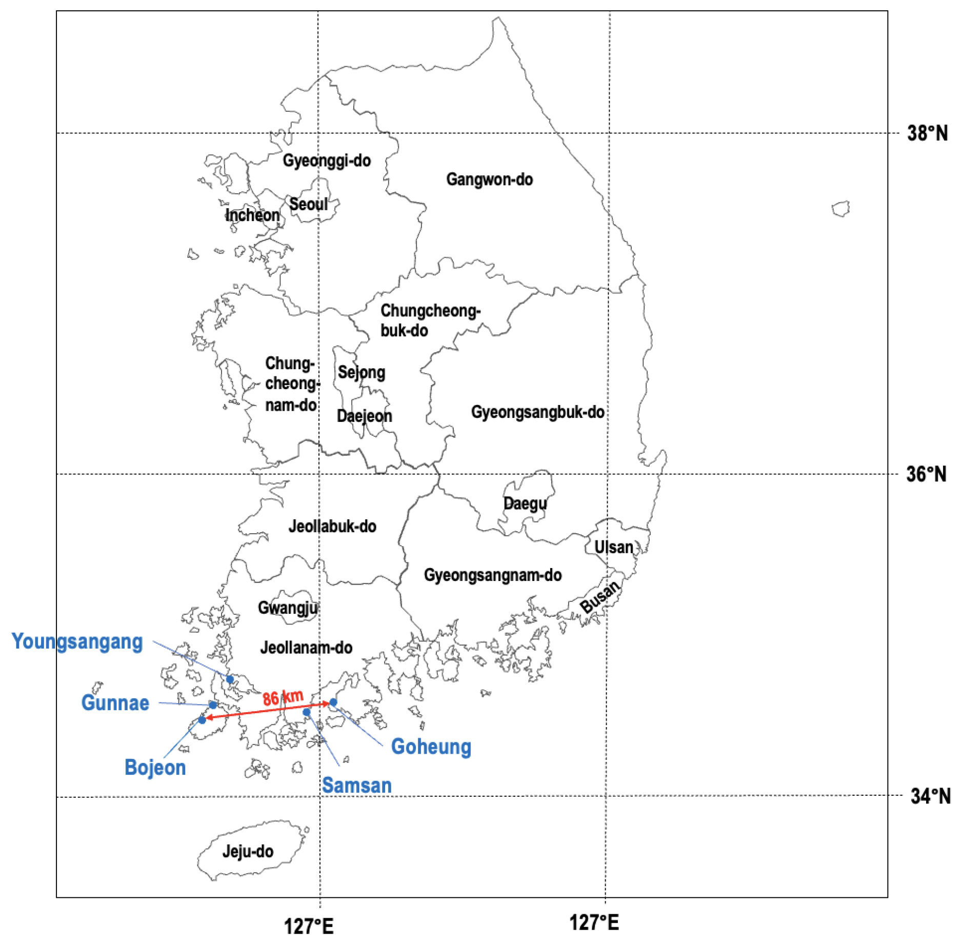
본 연구에서는 간척지 토양의 탄소 함량 예측을 위한 Random Forest 모델 적용 가능성을 검증하기 위하여 우리나라 간척지 토양의 이화학성을 조사한 Park et al. (2022)의 결과 일부를 활용하였다 (Table 2). Park et al. (2022)은 우리나라 서남해안에 위치한 간척지 36개 필지 (고흥 9개, 군내 7개, 보전 3개, 삼산 5개, 영산강 지구 12개)의 토성 (모래, 실트 및 점토 함량)과 pH, ECe, ESP, SAR (sodium absorption ratio; 나트륨 흡착비), CEC (cation exchange capacity; 양이온교환용량), 교환성 (Na+) 및 수용성 (Na+, Ca2+, Mg2+) 양이온 함량, 토양 양분 (무기태 질소 (NH4+, NO3-, NH4++NO3-)와 유효 인산) 및 유기 탄소 함량 등 총 17개의 항목을 조사하였다.

Park et al. (2022)이 조사한 간척지 필지는 반경 약 43 km 이내에 위치하고 있으며 (Fig. 2), 평균 기온 14.0°C, 강수량 1,455.6 mm로 기후 조건이 유사하였다 (KMA, 2018). 또한, 조사 대상 간척지 필지는 모두 경사가 없는 지형에서 벼 재배에 이용되고 있었다 (Park et al., 2022). 토양 유기 탄소 함량과 토양 특성의 상관관계는 IBM SPSS Statistics 26 (IBM Crop., Armonk, New York, USA)의 상관분석을 이용하여 평가하였으며, 95% 수준에서 유의성을 검토하였다.

Table 2.

Descriptive statistics for soil data of reclaimed tideland (RTL) soils used for random forest model.

Soil
properties
Sand
(%)
Silt
(%)
Clay
(%)
CEC
(cmolc
kg-1)
pH ECe
(dS m-1)
ESP
(%)
SAR Exc.
Na+
(cmolc
kg-1)
Sol.
Na+
(mmolc
kg-1)
Sol.
Ca2+
(mmolc
kg-1)
Sol.
Mg2+
(mmolc
kg-1)
NH4+
(mg N
kg-1)
NO3-
(mg N
kg-1)
NH4+
+ NO3-
(mg N
kg-1)
Avail.
P
(mg P
kg-1)
Orga-
nic C
(g kg-1)
Bojeon RTL
Number 3 3 3 3 3 3 3 3 3 3 3 3 3 3 3 3 3
Mean 47.5 38.5 14.1 7.8 7.2 7.9 18.3 5.1 1.4 6.5 0.9 2.5 15.7 17.2 33.0 5.2 11.1
SD 8.5 6.9 1.9 1.1 1.0 2.4 1.7 1.8 0.1 2.0 0.7 0.5 6.2 29.9 36.0 2.8 0.2
Minimum 42.2 30.6 12.1 6.9 6.2 5.2 16.3 3.6 1.3 5.0 0.1 2.0 11.4 0.0 11.4 3.4 10.9
Maximum 57.3 43.8 16.0 9.1 8.1 9.9 19.5 7.1 1.5 8.8 1.5 3.1 22.9 51.7 74.6 8.5 11.4
Goheung RTL
Number 9 9 9 9 9 9 9 9 9 9 9 9 9 9 9 9 9
Mean 17.0 63.9 19.1 10.6 8.2 10.4 15.3 6.2 1.6 7.3 1.0 2.4 11.6 23.6 35.2 6.2 8.9
SD 13.1 11.9 4.3 2.1 0.4 2.3 2.8 3.1 0.1 2.1 0.6 0.8 5.1 28.0 28.1 2.3 1.6
Minimum 3.4 41.4 12.1 8.0 7.6 7.6 10.9 2.5 1.5 3.9 0.1 1.1 2.9 0.0 2.9 3.5 6.9
Maximum 46.5 75.6 25.2 14.0 8.6 14.3 19.4 12.9 1.6 10.2 1.8 3.5 17.9 78.2 93.1 11.1 11.6
Gunnae RTL
Number 7 7 7 7 7 7 7 7 7 7 7 7 7 7 7 7 7
Mean 8.5 62.6 28.9 14.2 7.6 8.3 10.9 2.7 1.5 4.1 1.7 3.3 15.7 2.3 18.0 2.3 11.9
SD 4.3 7.2 7.5 2.8 0.6 1.4 1.6 1.5 0.1 2.1 0.6 1.2 2.7 4.0 3.5 1.2 3.0
Minimum 3.8 53.9 17.6 12.0 6.7 6.8 8.0 0.7 1.4 1.2 1.1 1.0 12.6 0.0 13.4 0.9 8.7
Maximum 15.5 73.6 41.9 19.7 8.3 10.5 12.4 4.4 1.6 7.1 2.5 4.6 20.6 11.0 23.5 4.3 15.8
Samsan RTL
Number 5 5 5 5 5 5 5 5 5 5 5 5 5 5 5 5 5
Mean 35.0 50.0 15.0 7.7 8.4 14.9 23.8 4.1 1.4 8.0 3.0 4.3 7.2 24.4 31.7 12.5 6.6
SD 7.6 11.6 5.8 3.3 0.1 13.5 18.6 2.8 0.5 6.4 1.2 2.0 1.9 32.0 32.3 13.8 3.7
Minimum 24.1 40.8 6.0 2.9 8.3 3.1 5.0 1.7 0.6 3.4 1.3 2.4 4.9 0.0 4.9 2.4 3.0
Maximum 45.7 69.9 21.6 11.1 8.5 37.0 54.5 8.4 1.7 16.5 4.1 7.4 9.9 80.3 87.6 35.0 11.0
Youngsangang RTL
Number 12 12 12 12 12 12 12 12 12 12 12 12 12 12 12 12 12
Mean 21.2 46.2 32.6 12.6 7.4 9.0 13.9 7.9 1.6 8.3 0.5 2.1 16.5 5.4 21.9 6.0 10.1
SD 21.5 16.2 7.7 3.3 1.1 2.9 4.2 3.5 0.0 2.5 0.4 1.0 6.5 6.4 9.1 3.4 2.9
Minimum 0.6 13.6 18.9 7.0 4.9 5.0 9.3 3.3 1.5 5.2 0.0 1.0 6.4 0.0 8.5 1.7 4.3
Maximum 65.5 71.9 43.9 17.6 8.7 17.0 22.9 15.8 1.7 12.9 1.8 4.6 26.1 19.3 37.5 12.5 14.2
Total
Number 36 36 36 36 36 36 36 36 36 36 36 36 36 36 36 36 36
Mean 21.8 53.7 24.5 11.3 7.8 9.9 15.4 5.7 1.5 7.1 1.2 2.8 13.8 13.0 26.8 6.2 9.8
SD 17.9 15.0 9.7 3.5 0.9 5.5 8.0 3.4 0.2 3.3 1.0 1.3 5.8 21.3 21.2 6.0 3.0
Minimum 0.6 13.6 6.0 2.9 4.9 3.1 5.0 0.7 0.6 1.2 0.0 1.0 2.9 0.0 2.9 0.9 3.0
Maximum 65.5 75.6 43.9 19.7 8.7 37.0 54.5 15.8 1.7 16.5 4.1 7.4 26.1 80.3 93.1 35.0 15.8

CEC, cation exchange capability; ESP, exchangeable sodium percentage; SAR, sodium absorption ratio; Exc., exchangeable; Sol., soluble; Avail., available.

https://static.apub.kr/journalsite/sites/ksssf/2022-055-01/N0230550107/images/ksssf_55_01_07_F2.jpg
Fig. 2.

Geographical locations of the reclaimed tidelands for application of random forest models.

Random Forest 모델 검증

본 연구에서는 토양 유기 탄소 함량을 제외한 16개의 토양 이화학성 항목을 독립 변수로 설정하고 Random Forest 회귀 모델을 구동하여 토양 유기 탄소 함량을 예측하였다. 총 36개 (필지 수)의 데이터에 대하여 8:2의 비율로 무작위로 분리하여 Random Forest 회귀 모델을 구동하고 검증하였다 (Table 3). 과적합 방지와 예측 정확도 향상을 위해 의사결정 나무의 개수 (n_estimator)는 4개, 의사결정 나무의 최대 깊이 (max_depth)는 3, 잎 줄기의 최소 샘플 개수 (min_samples_split)는 1개, 줄기의 최소 개수 (min_samples_leaf)는 0.15개로 하이퍼 파라미터를 지정하였으며, 지정한 하이퍼 파라미터는 ‘GridSearchCV’ 모듈을 통해 여러 옵션들을 탐색하여 찾은 최적 값을 이용하였다 (Table 4). 특히, 본 연구에서는 의사결정 나무의 개수의 최적 값이 4개로 타 연구 (대부분 200 - 1,000개)에 비해 현저히 낮았다 (Hastie et al., 2009). 모델의 정확성 평가에는 평균 제곱 오차 (root mean square error, RMSE)와 결정 계수 (R2)를 사용하였다.

Table 3.

Descriptive statistics for training and test data used to build and validate random forest model.

Soil
properties
Sand
(%)
Silt
(%)
Clay
(%)
CEC
(cmolc
kg-1)
pH ECe
(dS m-1)
ESP
(%)
SAR Exc.
Na+
(cmolc
kg-1)
Sol.
Na+
(mmolc
kg-1)
Sol.
Ca2+
(mmolc
kg-1)
Sol.
Mg2+
(mmolc
kg-1)
NH4+
(mg N
kg-1)
NO3-
(mg N
kg-1)
NH4+
+ NO3-
(mg N
kg-1)
Avail.
P
(mg P
kg-1)
Orga-
nic C
(g kg-1)
Training data
Number 28 28 28 28 28 28 28 28 28 28 28 28 28 28 28 28 28
Mean 21.5 54.0 24.5 11.2 7.8 9.4 16.1 5.9 1.7 7.1 1.2 2.8 14.3 11.4 25.7 6.5 9.6
SD 19.2 15.9 10.3 3.9 0.9 3.0 8.6 3.6 0.1 3.0 1.0 1.4 6.3 18.3 19.4 6.6 2.7
Minimum 0.6 13.6 6.0 2.9 4.9 5.0 8.0 0.7 1.3 1.2 0.1 1.0 2.9 0.0 2.9 0.9 4.3
Maximum 65.5 75.6 43.9 19.7 8.7 18.1 54.5 15.8 1.7 13.3 4.1 7.4 26.1 78.2 93.1 35.0 15.8
Test data
Number 8 8 8 8 8 8 8 8 8 8 8 8 8 8 8 8 8
Mean 22.9 52.6 24.5 11.6 7.7 11.6 12.9 5.1 1.4 6.8 1.5 2.6 11.9 18.6 30.4 5.0 10.4
SD 13.5 12.0 7.7 2.2 0.9 10.6 4.3 2.8 0.4 4.6 1.2 1.0 3.5 30.6 27.8 3.3 3.9
Minimum 6.5 39.6 15.9 8.3 6.2 3.1 5.0 1.4 0.6 2.4 0.0 1.2 7.4 0.0 11.4 2.3 3.0
Maximum 42.9 72.0 35.6 14.3 8.5 37.0 19.9 8.4 1.7 16.5 3.3 4.5 16.5 80.3 87.8 12.5 15.6

CEC, cation exchange capability; ESP, exchangeable sodium percentage; SAR, sodium absorption ratio; Exc., exchangeable; Sol., soluble; Avail., available.

Table 4.

Options for each hyper parameter used in ‘GridSearchCV’ module to search for optimal hyper parameters.

Hyper parameter Options
n_estimators 4, 7, 10, 20, 50, 75, 100, 250, 500
max_depth 1, 3, 5, 7, 10, 12, 15
min_samples_split 1, 2, 4, 6, 8, 10
min_samples_leaf 0.1, 0.15, 0.2, 0.25, 0.3, 0.5, 0.7, 1.0

Results and Discussion

Random Forest 모델의 정확도

Random Forest 모델 학습에 총 36개의 필지 중 28개 필지의 토양 특성 데이터가 사용되었으며, 나머지 8개 필지의 토양 특성 데이터는 모델 검증에 사용되었다 (Table 3). 학습에 사용된 28개 필지의 토양 탄소 함량은 4.3 - 15.8 g kg-1 (평균 9.6 g kg-1)의 범위였으며, 검증에 사용된 8개 필지의 토양 유기 탄소 함량은 3.0 - 15.6 g kg-1 (평균 10.4 g kg-1)의 범위였다.

Random Forest 모델을 통해 예측한 토양 탄소 함량 (예측 값)과 Park et al. (2022)이 조사한 토양 탄소 함량 (실측 값)을 비교한 결과, 그 차이는 평균 25.9%였다 (Fig. 3a). 하지만, 실측 값이 학습한 데이터의 범위를 벗어나거나 최소 (4.3 g kg-1)/최댓값 (15.8 g kg-1)에 근접할 경우 (3번과 6번 시료), 예측 값 (각각 10.6, 6.4 g kg-1)과 실측 값 (각각 15.6, 3.0 g kg-1)의 차이는 평균 73.9%였다 (Table 3Fig. 3). 이는 Random Forest 모델이 학습한 데이터의 범위 내에서만 값을 예측할 수 있기 때문이다 (Breiman, 2001). 따라서, 모델의 정확도를 향상하기 위해서는 가급적 많은 양의 데이터를 이용하여 넓은 범위의 데이터를 학습시키는 것이 필요하다. 실측 값이 학습한 데이터의 범위 내에 포함될 경우, 예측 값과 실측 값의 차이가 평균 9.9%로 감소하였다 (Fig. 3a). 모델의 정확도는 검증 방식 (leave-one-out cross validation, out-of-bag, cross-validation 등)에 따라 달라질 수 있지만 (Yao et al., 2019; Calle et al., 2021), 본 연구에서 구현된 Random Forest 모델은 RMSE = 2.13, R2 = 0.67로 정확도가 통계적으로 유의하였다 (Fig. 3b). 따라서, 본 연구 결과를 통해 간척지 토양 탄소 함량을 예측하는데 Random Forest 모델의 활용 가능성을 확인하였다.
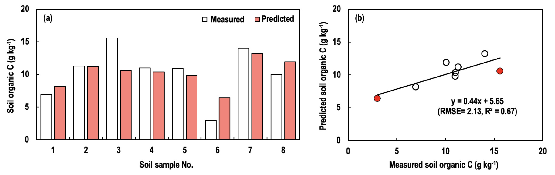
https://static.apub.kr/journalsite/sites/ksssf/2022-055-01/N0230550107/images/ksssf_55_01_07_F3.jpg
Fig. 3.

Random forest modeling results: (a) A bar graph showing the values predicted by the random forest model and measured by Park et al. (2022) and (b) correlation between the values measured and predicted. Soil organic carbon (C) contents were predicted using 20% of the total data (i.e., 8 soil samples) in the process of validating the random forest model. The red circles indicate that the investigated values were out of the range of the learned data or those were close to the minimum or maximum value of the learned data.

토양 탄소 함량 예측에 대한 주요 토양 특성 변수

Random Forest 모델은 타 기계학습 기반의 예측 모델과 달리 예측에 영향을 미치는 독립 변수의 기여도를 확인할 수 있다는 장점이 있다 (Breiman, 2001). 간척지 토양의 탄소 함량을 예측하기 위한 가장 중요한 토양 특성 변수는 토양의 NH4+ 함량 (기여도 14.9%)이었으며, CEC (14.7%), NH4+ + NO3- 함량 (14.4%), pH (13.2%), 수용성 Mg2+ 함량 (10.6%) 등의 순서였다 (Fig. 4). 토양 탄소는 작물의 생산성과 미생물 호흡에 의한 손실, 그리고 토양 구성 성분과의 상호작용에 의한 안정화 등 매우 다양한 요인에 영향을 받기 때문에 (Wiesmeier et al., 2019; Park et al., 2022) 개별 지표의 기여도의 인과 관계는 현 단계에서 불명확하다. 그럼에도 불구하고, 양분 함량과 CEC의 기여도가 높은 것은 토양 양분과 이화학성, 작물 바이오매스, 그리고 토양 탄소의 상관관계를 반영하는 것으로 해석된다 (Lim et al., 2020; Park et al., 2022).

하지만, Random Forest 모델을 통해 파악된 주요 토양 특성 변수는 토양 탄소 함량에 대한 토양 특성의 상관성과 관계가 없었다 (Table 5Fig. 4). 특히, ECe의 경우, 토양 탄소 함량과 가장 상관성 (R2 = 0.29, P = 0.001)이 높은 토양 특성임에도 불구하고 Random Forest 모델에서 기여도가 0%였다 (Table 5Fig. 4). 이상의 연구 결과는 본 연구의 가설과 상반되는데, 이는 예측하고자 하는 필지의 ECe 실측 값 일부가 Random Forest 모델을 구현하기 위해 학습한 ECe의 범위를 벗어나거나 최소/최댓값에 근접하였기 때문으로 판단된다 (Table 3). ECe 뿐만 아니라 기여도가 낮은 변수 대부분 (ESP, 교환성 Na+ 함량, 수용성 Na+ 및 Ca2+ 함량, NO3- 함량)의 실측 값이 학습한 데이터의 범위를 벗어났다 (Table 3). 따라서, 본 연구 결과는 모델의 예측 정확도를 위해서는 사용되는 데이터의 수와 범위가 중요함을 제시한다.

일반적으로 기여도가 낮은 변수를 제거하여 Random Forest 모델을 구현하면 모델의 정확도가 향상된다 (Breiman, 2001). 하지만, 본 연구에서는 기여도가 0%인 변수를 제거하고 모델을 구현하였을 때 모델의 RMSE = 2.61, R2 = 0.52이였으며, 실측 값과 예측 값은 평균 29.6%의 차이로 정확도가 더 낮아졌다 (Fig. 5). 이는 본 연구에서 사용된 데이터의 수가 타 연구들에 비해 상대적으로 적기 때문으로 판단된다. 따라서, 관련 D/B를 확대 구축하고 다양한 독립변수를 활용하여 모델을 구동한다면 모델의 예측 정확도를 향상시킬 수 있을 것으로 기대된다.
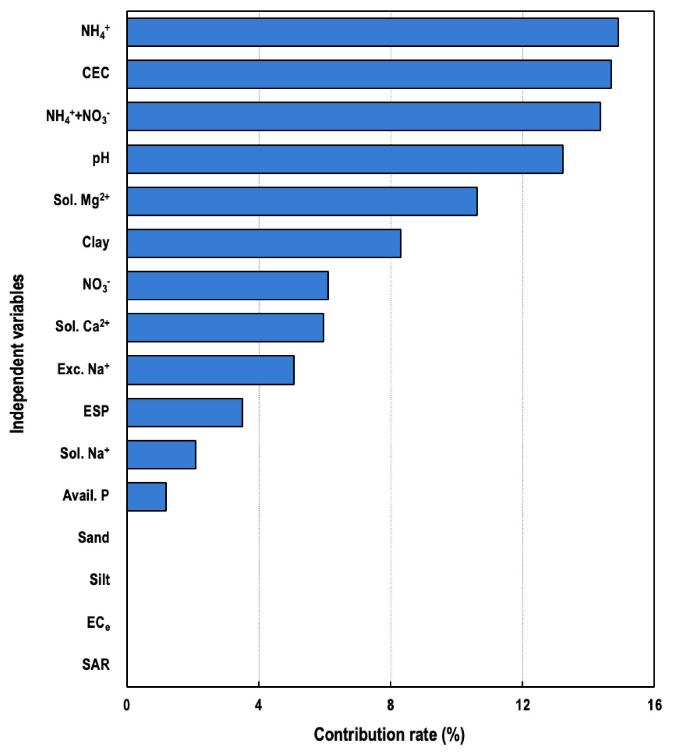
https://static.apub.kr/journalsite/sites/ksssf/2022-055-01/N0230550107/images/ksssf_55_01_07_F4.jpg
Fig. 4.

Contribution of independent variables to predict soil carbon contents. Details of independent variables are described in Table 2.

Table 5.

Correlations between soil organic C and soil properties used for independent variables.
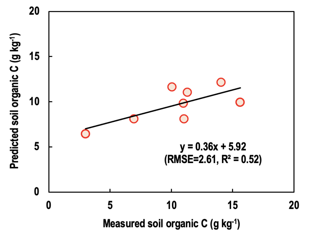
Independent variablesP values R2‡
Sand 0.569 0.01 (-)
Silt 0.533 0.01 (-)
Clay 0.037 0.12 (+)
CEC 0.013 0.17 (+)
pH 0.066 0.10 (-)
ECe0.001 0.29 (-)
ESP 0.005 0.21 (-)
SAR 0.810 0.00 (-)
Exc. Na+ 0.390 0.02 (-)
Sol. Na+ 0.164 0.06 (-)
Sol. Ca2+ 0.060 0.10 (-)
Sol. Mg2+ 0.216 0.04 (-)
NH4+0.001 0.27 (+)
NO3-0.038 0.12 (-)
NH4+ + NO3- 0.184 0.05 (-)
Avail. P 0.040 0.12 (-)

CEC, cation exchange capability; ESP, exchangeable sodium percentage; SAR, sodium absorption ratio; Exc., exchangeable; Sol., soluble; Avail., available.

The mark in parentheses means relationship between soil organic C and soil properties used for independent variables.

https://static.apub.kr/journalsite/sites/ksssf/2022-055-01/N0230550107/images/ksssf_55_01_07_F5.jpg
Fig. 5.

Correlation between values measured by Park et al. (2022) and predicted by the random forest model built by excluding the independent variables with 0% contribution to the prediction of soil carbon (C) contents. Soil organic C contents were predicted using 20% of the total data (i.e., 8 soil samples) in the process of validating the random forest model.

Conclusions

Random Forest 모델은 자연계의 복잡한 환경요인을 잘 반영하기 때문에 토양 탄소 함량 예측 연구에 적합하지만, 우리나라 토양의 탄소 함량을 예측하는데 활용된 사례가 매우 적다. 본 연구에서 우리나라 간척지 토양의 특성 조사 결과를 활용하여 Random Forest 모델을 구현한 결과, 높은 정확도로 토양 탄소 함량을 예측하였다. 하지만, 모델을 구현하기 위해 학습한 데이터의 수와 범위의 한계로 인해 일부 예측 값의 정확도가 낮았다. Random Forest 모델은 다른 기계학습 기반의 예측 모델에 비해 정확도가 높은 편이지만, 학습한 데이터의 범위 내에서만 예측이 가능하다는 단점이 있다. 따라서, 본 연구에서는 간척지 토양 탄소 함량 예측 연구를 위한 Random Forest 모델의 적용 가능성을 확인하였지만, 정확도 개선을 위해서는 많은 양의 데이터 축적 필요성이 제기되었다.

Acknowledgements

This work was carried out with the support of the “Cooperative Research Program of Agriculture Science and Technology Development (Project No. PJ0138732021)”, Rural Development Administration, Republic of Korea.

References

1
Ahn, B.K., D.Y. Ko, H.J. Choi, and H.G. Chon. 2020. Distribution of water-soluble nutrients and physico-chemical properties of upland and orchard field soils in Jeonbuk province. Korea J. Soil Sci. Fert. 53:375-381. 10.7745/KJSSF.2020.53.3.375
2
Breiman, L. 2001. Random forests. Mach. Learn. 45:5-32. 10.1023/A:1010933404324
3
Calle, J.L.P., M. Ferreiro-Gonzalez, A. Ruiz-Rodriguez, G.F. Barbero, J.A. Alvarez, M. Palma, and J. Ayuso. 2021. A methodology based on FT-IR data combined with random forest model to generate spectralprints for the characterization of high-quality vinegars. Foods 10:1141. 10.3390/foods1006141134207095PMC8233915
4
Chaplot, V., M. Bernoux, C. Walter, P. Curmi, and U. Herpin. 2001. Soil carbon storage prediction in temperate hydromorphic soils using a morphologic index and digital elevation model. Soil Sci. 166:48-60. 10.1097/00010694-200101000-00008
5
Florinsky, I.V., R.G. Eilers, G. Manning, and L. Fuller. 2002. Prediction of soil properties by digital terrain modelling. Environ. Modell. Software 17:295-311. 10.1016/S1364-8152(01)00067-6
6
Franklin, J. 2005. The elements of statistical learning: data mining, inference and prediction. Math. Intell. 27:83-85. 10.1007/BF02985802
7
Grimm, R., T. Behrens, M. Märker, and H. Elsenbeer. 2008. Soil organic carbon concentrations and stocks on Barro Colorado Island-Digital soil mapping using random forests analysis. Geoderma 146:102-113. 10.1016/j.geoderma.2008.05.008
8
Hastie, T., R. Tibshirani, J.H. Friedman, and J.H. Firedman. 2009. The elements of statistical leargnin: data mining, inference, and prediction. Springer, New York, USA.
9
Hwang, H.Y., S.H. Kim, M.S. Kim, D.W. Le, J.E. Rim, J.H. Shim, and S.J. Park. 2019. Soil organic carbon fractions and stocks as affected by organic fertilizers in rice paddy soil. Korean J. Soil Sci. Fert. 52:520-529. 10.7745/KJSSF.2019.52.4.520
10
Jeong, G.Y. 2018. Spatial prediction and economic evaluation of soil carbon stocks using digital soil mapping in an agricultural landscape. Geogr. J. Korea 52:389-401.
11
Karhu, K., A.I. Gärdenäs, J. Heikkinen, P. Vanhala, M. Tuomi, and J. Liski. 2012. Impacts of organic amendements on carbon stocks of an agricultural soil-Comparison of model-simulations to measurements. Geoderma 189:606-616. 10.1016/j.geoderma.2012.06.007
12
Kim, H.J., S.K. Kim, S.W. Kim, K.J. Kwak, and O.D. Kwon. 2021. Changes in chemical properties of orchard soils in Jeonnam province between 2002 and 2018. Korean J. Soil Sci. Fert. 54:1-9. 10.7745/KJSSF.2021.54.1.001
13
Kim, J. and S. Grunwald. 2016. Assessment of carbon stocks in the topsoil using random forest and remote sensing images. J. Environ. Qual. 45:1910-1918. 10.2134/jeq2016.03.007627898790
14
KMA (Korea Meteorological Administration). 2018. Annual climatological reports. Seoul, Korea.
15
Lal, R. 2008. Carbon sequestration. Philos. Trans. R. Soc. B: Biol. Sci. 363:815-830. 10.1098/rstb.2007.218517761468PMC2610111
16
Lee, J.H., J.H. Im, K.M. Kim, and J. Heo. 2015. Change analysis of aboveground forest carbon stocks according to the land cover change using multi-temporal Landsat TM images and machine learning algorithms. J. Korean Assoc. Geogr. Inf. Stud. 18:81-99. 10.11108/kagis.2015.18.4.081
17
Lee, Y.H., M.S. Kim, S.J. Park, H.Y. Hwang, and S.H. Kim. 2020. Assessment of soil organic carbon fractions and stocks under different farming practice in a single maize cropping system. Korean J. Soil Sci. Fert. 53:626-634. 10.7745/KJSSF.2020.53.4.626
18
Lim, S.S., H.I. Yang, H.J. Park, S.I. Park, B.S. Seo, K.S. Lee, S.H. Lee, S.M. Lee, H.Y. Kim, and J.H. Ryu. 2020. Land-use management for sustainable rice production and carbon sequestration in reclaimed coastal tideland soils of South Korea: A review. Soil Sci. Plant Nutr. 66:60-75. 10.1080/00380768.2019.1674121
19
Nabiollahi, K., S. Eskandari, R. Taghizadeh-Mehrjardi, R. Kerry, and J. Triantafilis. 2019. Assessing soil organic carbon stocks under land-use change scenarios using random forest models. Carbon Manag. 10:63-77. 10.1080/17583004.2018.1553434
20
Nguyen, T.T., T.D. Pham, C.T. Nguyen, J. Delfos, R. Archibald, K.B. Dang, N.B. Hoang, W. Guo, and H.H. Ngo. 2022. A novel intelligence approach based active and ensemble learning for agricultural soil organic carbon prediction using multispectral and SAR data fusion. Sci. Total Environ. 804:150187. 10.1016/j.scitotenv.2021.15018734517328
21
Park, H.J., B.S. Seo, Y.J. Jeong, H.I. Yang, S.I. Park, N.R. Baek, J.H. Kwak, and W.J. Choi. 2022. Soil salinity, fertility and carbon content, and rice yield of salt-affected paddy with different cultivation period in southwestern coastal area of South Korea. Soil Sci. Plant Nutr. 10.1080/00380768.2021.1967082.
22
Powers, J.S. and W.H. Schlesinger. 2002. Relationships among soil carbon distributions and biophysical factors at nested spatial scales in rain forests of northeastern Costa Rica. Geoderma 109:165-190. 10.1016/S0016-7061(02)00147-7
23
Schmidt, M.W., M.S. Torn, S. Abiven, T. Dittmar, G. Guggenberger, I.A. Janssens, M. Kleber, I. Kögel-Knabner, J. Lehmann, and D.A. Manning. 2011. Persistence of soil organic matter as an ecosystem property. Nature 478:49-56. 10.1038/nature1038621979045
24
Smith, P. 2012. Soils and climate change. Curr. Opin. Environ. Sustainability 4:539-544. 10.1016/j.cosust.2012.06.005
25
Sothe, C., A. Gonsamo, J. Arabian, and J. Snider. 2022. Large scale mapping of soil organic carbon concentration with 3D machine learning and satellite observations. Geoderma 405:115402. 10.1016/j.geoderma.2021.115402
26
Thompson, J.A. and R.K. Kolka. 2005. Soil carbon storage estimation in a forested watershed using quantitative soil-landscape modeling. Soil Sci. Soc. Am. J. 69:1086-1093. 10.2136/sssaj2004.0322
27
Thompson, J.A., E.M. Pena-Yewtukhiw, and J.H. Grove. 2006. Soil-landscape modeling across a physiographic region: Topographic patterns and model transportability. Geoderma 133:57-70. 10.1016/j.geoderma.2006.03.037
28
Wang, B., J.M. Gray, C.M. Waters, M.R. Anwar, S.E. Orgill, A.L. Cowie, P. Feng, and D.L. Liu. 2022. Modelling and mapping soil organic carbon stocks under future climate change in south-eastern Australia. Geoderma 405:115442. 10.1016/j.geoderma.2021.115442
29
Wiesmeier, M., L. Urbanski, E. Hobley, B. Lang, M. von Lützow, E. Marin-Spiotta, B. van Wesemael, E. Rabot, M. Ließ, and N. Garcia-Franco. 2019. Soil organic carbon storage as a key function of soils-A review of drivers and indicators at various scales. Geoderma 333:149-162. 10.1016/j.geoderma.2018.07.026
30
Yao, D., X. Zhan, and C.K. Kwoh. 2019. An improvved random forest-based computational model for predicting novel miRNA-disease associations. BMC Bioinformatics 20:1-14. 10.1186/s12859-019-3290-731795954PMC6889672
31
Zeraatpisheh, M., Y. Garosi, H.R. Owliaie, S. Ayoubi, R. Taghizadeh-Mehrjardi, T. Scholten, and M. Xu. 2022. Improving the spatial prediction of soil organic carbon using environmental covariates selection: A comparison of a group of environmental covariates. Catena 208:105723. 10.1016/j.catena.2021.105723
32
Zhou, T., Y. Geng, J. Chen, M. Liu, D. Haase, and A. Lausch. 2020. Mapping soil organic carbon content using multi-source remote sensing variables in the Heihe River Basin in China. Ecol. Indic. 114:106288. 10.1016/j.ecolind.2020.106288
페이지 상단으로 이동하기